How to Quickly Create Percentage Change Formulas with a Macro

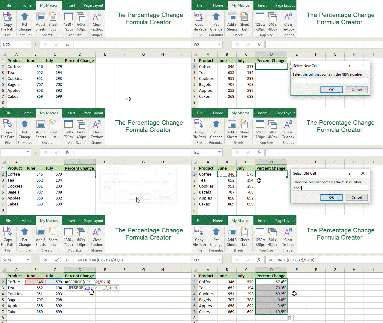
Bottom line: Percentage change formulas require a lot of typing to create a simple calculation.  This macro will create the entire formula for you, including the IFERROR function.

Skill level: Intermediate

The image above is an animated screencast.  Click here to view it in your web browser.

Download the File

Download the Excel file to follow along.

The Percentage Change Formula Explained

To calculate the percentage change between two numbers we typically write a formula like the following:

=(C2-B2)/B2

Whenever I am creating this formula I always think, “new minus old, divided by old”.  Or:

=(new value – old value) / old value

If we want to handle/prevent any divide by zeros (#DIV/0!), then we can wrap the formula in the IFERROR function.

=IFERROR((C2-B2)/B2,0)

The formula above would return a zero if the denomiator (A1/old value) is zero.

This formula can also be used to calculate discount percentages, so you can use it when you are shopping.  

discount % = (new discounted price – old regular price) / old regular price

Simplified Formula

The formula can also be simplified to:

=(new value / old value) – 1

This will return the same result as the other formula.  The formula you use is a matter of personal preference, or your boss's preference. 🙂  Thanks to XLArium for mentioning this is the comments.

Either way, there are a ton of different uses for the percentage change formula. It's one that should be in every Excel user's toolbox.

The Percent Change Formula Creator Macro

The percentage change formula isn't too terribly long, but it can take some time to type out.  So I wrote this simple macro that will write the formula for us.

Here's how it works…

1. The macro uses the InputBox method, and asks you to select the cells that contain the new and old values.
2. It then writes the percentage change formula, including the IFERROR function, and puts the formula in the ActiveCell.

It's a super simple time saver for a very common formula. 🙂

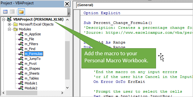
Here is the VBA code.  You can copy/paste it to your personal macro workbook.

Sub Percent_Change_Formula()
'Description: Creates a percentage change formula
'Source: https://www.excelcampus.com/vba/percentage-change-formulas-macro/

Dim rOld As Range
Dim rNew As Range
Dim sOld As String
Dim sNew As String
Dim sFormula As String
    
    'End the macro on any input errors
    'or if the user hits Cancel in the InputBox
    On Error GoTo ErrExit
    
    'Prompt the user to select the cells
    Set rNew = Application.InputBox( _
            "Select the cell that contains the NEW number", _
            "Select New Cell", Type:=8)
    Set rOld = Application.InputBox( _
            "Select the cell that contains the OLD number", _
            "Select Old Cell", Type:=8)
    
    'Get the cell addresses for the formula - relative references
    sNew = rNew.Address(False, False)
    sOld = rOld.Address(False, False)
        
    'Create the formula
    sFormula = "=IFERROR((" & sNew & " - " & sOld & ")/" & sOld & ",0)"

    'Create the formula in the activecell
    ActiveCell.Formula = sFormula
    
ErrExit:
    
End Sub

It's important to note that this macro will override the value or formula in the activecell with the result.  We can add additional code to prevent that.  More on that below.

How to Use the Macro

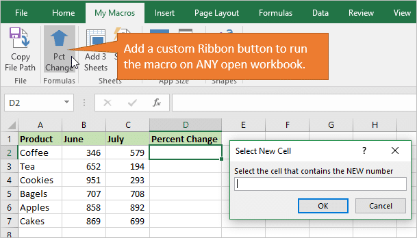
I put this macro in my Personal Macro Workbook, and then create a ribbon button and/or keyboard shortcut for it.  You could also put it in an add-in file.

Either of these options will allow you to use the macro on any Excel file you have open.  This means that you do NOT have to copy/paste the code to each file you want to use it in.  You can put it in your Personal Macro Workbook, and use it on ANY file.

Here is a screencast of the macro in action.  You can see how simple it is to create the formula.  All you have to do is click a few buttons and select two cells.  No typing required! 🙂

Checkout my article and video series on the Personal Macro Workbook for details on how to set this up and create custom ribbon buttons to run your macros.

Other Options for the Percentage Change Macro

The possibilities are pretty much endless for this macro.  You can change it to fit your needs.  Here are a few things we could change:

• Change the value_if_error value from 0 (zero) to another value.
• Remove the IFERROR function completely.
• Warn the user before putting the formula in the active cell.
• Copy the formula to the clipboard instead of putting it in the active cell.
• Format the active cell with a percentage format.
  Code: ActiveCell.NumberFormat = “0.0%”

What other changes would you like to make?  Please leave a comment below with your suggestions or questions.  Thanks! 🙂