Bottom line: Learn how to create percentage change formulas in Excel with negative numbers.
Skill level: Intermediate
In my last post I shared a macro to quickly create percentage change formulas. I also explained two formulas we can use to calculate percentage change.
Formula #1
=(new value – old value) / old value
Formula #2
=(new value / old value) – 1
Both of these formulas will produce the same result when the numbers are positive. The one you use is just a matter of personal preference.
The goal of the percentage change formula is to allow us to make comparisons on performance between two or more items. This could be time periods, entities, categories, businesses, etc. This formula can also be used to calculate discount percentages.
Download the File
Download the file to follow along.
What if the numbers are Negative?
After a bit of research, I have not found a good way to calculate the percentage change when either the old number or the new number are negative. There are definitely formulas you can use, but they seem to produce incorrect or misleading results.
The Wall Street Journal has an old guide to earnings reports that says this:
Net Income percent change is the change from the same period from a year ago. Percent change is not provided if either the latest period or the year-ago period contains a net loss [negative number]. On the digest page, if a company posts a profit in the latest period against a loss in the year-ago period, the percent change is represented as a “P”. Similarly, if a company posts a loss in the latest period against a profit in the year-ago period, the percent change is represented as a “L”.
This article might be outdated, as I have found that recent WSJ financial pages are using the ABS method (more on that below) to calculate percentage change, but the point is that percentage change on negative numbers can produce misleading results.
What about the ABS (Absolute) Method?
One common way to calculate percentage change with negative numbers it to make the denominator in the formula positive. The ABS function is used in Excel to change the sign of the number to positive, or its absolute value.
Here is the formula that is commonly used:
=(new value – old value) / ABS(old value)
Technically this formula works to produce a percentage change number with the correct sign (positive/negative). However, I believe it produces misleading results.
The image below contains an example of this. The Old value is negative and the New value is positive.
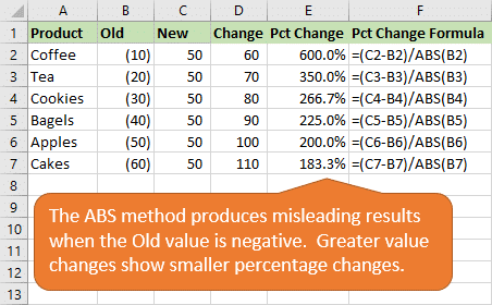
- When the value goes from -10 to 50, the amount change is +60 and percentage change is 600%.
- When the value goes from -60 to 50, the amount change is +110 and percentage change is 183.3%
Although the calculation is technically correct because we changed the denominator (old value) to a positive number, the results don't really make sense to me.
If you were just looking at the percentage change numbers, you would think that Coffee did better than Cakes. When in reality Cakes made a huge gain in profit over the prior period, much larger than Coffee.
The same issue happens when the numerator (new value) is negative. Here is another example that produces misleading results.
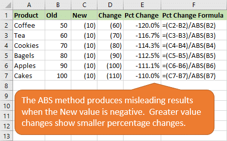
In this example Cakes had a larger negative value change, but smaller percentage change than Coffee.
But I've Always used the ABS Method!!!
I know, me too. I've seen this method used throughout my career, and it looks like the Wall Street Journal is even using it. I spotted it in some of their growth metrics on this page of Bank of America financials.
It's hard to say that it's completely wrong to use the ABS formula. But, it's good to know that the results might be misleading. So use it with caution! 😉
Alternate Calculations for Percentage Change with Negative Numbers
Here are a few ways to test for the presence of a negative number, and provide an alternate result.
Method #1: No Result for Negatives
The first thing we can do is check if either number is negative, and then display some text to tell the reader a percentage change calculation could not be made.
The following formula does this with an IF function and MIN function.
=IF(MIN(old value, new value)<=0,"--",(new value/old value)-1)
Here's how the formula works:
- The logical test of the IF function (MIN(old value, new value)<=0) finds the minimum of the two values and tests if the value is less than or equal to zero. The result will either be TRUE or FALSE.
- If the result is TRUE, then a negative number (or zero) exists. In this case we can display some text to tell the reader. This can be anything you want. I just used two dashes “–“. You could also have it return an N/A error with the NA() function, or any other text that lets the reader know the percentage change could not be calculated.
- If the result is FALSE, then the percentage change formula is used to return the percentage change on the two positive numbers.
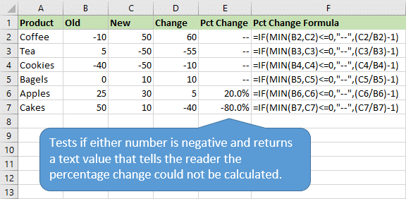
This formula also handles the divide by zero (#DIV/0!), so we don't have to wrap it in the IFERROR function.
Method #2: Show Positive or Negative Change
The Wall Street Journal guide says that its earning reports display a “P” or “L” if there is a negative number and the company posted a profit or loss.
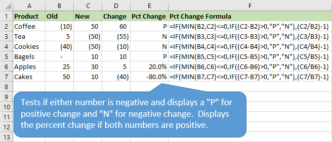
We could use this same methodology to tell our readers if the change was positive (P) or negative (N) when either value is negative.
The following formula tests for this with an additional IF function.
=IF(MIN(old value, new value)<=0,IF((new value - old value)>0,"P","N"),(new value/old value)-1)
Here's how the formula works:
- We start with the same logical test to determine if a negative value exists using the MIN function.
- A second IF function is then used to determine if the change from old to new is positive or negative.
IF((new value – old value)>0,”P”,”N”)
This IF statement returns a “P” for a positive change and an “N” for a negative change. - If both numbers are positive then the percentage change formula is used to display the result.
Other Methods for Percentage Change with Negatives?
Calculating the percentage change when negative numbers are involved is not easy. The ABS method is probably the most commonly used, but it can produce misleading results.
The ultimate goal should be to keep things positive, so we don't have to worry about the negative… 😉
Do you have any other methods for this calculation? Can we further simplify either of the methods above? I'm interested to hear your thoughts. Please leave a comment below with questions or suggestions. Thanks!


I could not find the good one above, so I designed my one.
This is my rendition :
=IFS( AND ( A1 >= 0, A1 1 , B1 / A1 – 1, A1 < 0 , ABS(A1) + B1 )
Just multiply the result of the standard arithmetic return shown in ‘Formula #2’ by the ‘sign’ (+1 or -1) of the ‘old value’.
Done.
just tried, had doubt with the abs method, agree with your opinion that it might be misleading, but believe that it can be fixed with an added element of “-1” when the base is negative
Hi, I based this formula on a post above by poster “jomili “. Although his formula worked well with most numbers (positive and negative), his formula did break when you had a combination of two negative numbers with a positive result (vs. a combination of two negative numbers with a negative result), which was the only remaining combination.
Here is the improved formula, enjoy. And thank you, jomili!
=IF(MIN(A13, B13)>0,(B13/A13)-1,
IF(AND(A13<=0,B13A13, ABS(ABS(B13)/ABS(A13)-1), ABS(ABS(B13)/ABS(A13)-1)*-1 ),
IF(A13<=0,(B13+ABS(A13)+2/2)-1,
-(ABS(B13)+A13+2/2)-1)))
A B Results
6 8.00 0.3333
5 8.00 0.6000
4 8.00 1.0000
3 8.00 1.6667
2 8.00 3.0000
1 8.00 7.0000
-1 8.00 9.0000
-2 -1.00 0.5000
-3 -1.00 0.6667
-3 -1.00 0.6667
-3 -2.00 0.3333
-6 -5.00 0.1667
-7 -8.00 -0.1429
-8 -9.00 -0.1250
-9 -10.00 -0.1111
-10 -11.00 -0.1000
-11 -12.00 -0.0909
Above are the results when "B" is compared to "A"
Updating for posterity, and for anyone who’s looking for a solution: my previous copy-paste gave me Excel errors. Anyways, here’s my reworked solution with proper negative assignments;
=IF(MIN(A2, B2)>0,(B2/A2)-1,
IF((A20,(ABS(ABS(B2)/ABS(A2)+1))*1,ABS(ABS(B2)/ABS(A2)-1)*1),
IF(A2>0, ((ABS(-ABS(B2)-ABS(A2))/ABS(A2))) *-1, ABS(ABS(B2)/ABS(A2)-1)*-1) ))
Beginning End Result
8 6 -0.25
6 -8 -2.33
-8 6 1.75
-8 -6 0.25
8 6 -0.25
-8 -10 -0.25
8 -10 -2.25
-1 -2 -1.00
-3 -2 0.33
-6 -5 0.17
-7 -8 -0.14
-8 -6 0.25
-8 -10 -0.25
wow, copy and paste doesn’t work well with text formulas on this website. Hopefully this works:
=IF(MIN(A2, B2)>0,(B2/A2)-1,
IF((A20,(ABS(ABS(B2)/ABS(A2)+1))*1,ABS(ABS(B2)/ABS(A2)-1)*1),
IF(A2>0, ((ABS(-ABS(B2)-ABS(A2))/ABS(A2))) *-1, ABS(ABS(B2)/ABS(A2)-1)*-1) ))”
great stuff, really helped as I was struggling with this issue too
I’ll save your time, the majority of the comments below completely miss the point the article is trying to make. I agree with the article and offer a small recommendation. If the value had no change, the formula Jay offers still would show positive or negative. If you want a formula that will show no change and also not show an error for dividing by zero, use this one:
=IF(NEW=OLD, “No Move”,IF(MIN(OLD,NEW)0,”Positive”,”Negative”),(NEW/OLD)-1))
Hi Jon,
I really appreciate the alternative solutions, but I am not sure I see the problem with the ABS method when the new number is negative but the old number is positive. The same “issue” would exist if both were positive numbers. a change value of 25 would be 50% change if the starting value was 50, but it would be only 25% if the starting value is 100. Which is what was happening with the negative new value case. Even though it was a greater absolute change the percent change is a relative value so the greater the starting value the lower the (relative) percent change. It doesn’t really have anything to do with new number being negative. However when the old number is negative I do agree that it can’t be evaluated the same. I feel this case is different than when the new value is negative. It appears that the relative comparison must be made to a positive value. I agree you need to be careful when evaluating percent change values in general so that you don’t necessarily think that the greatest percent change is equal to the greatest absolute change.
Or, did I miss the point of your concern about the results of using ABS() ? I am new to the program and just trying to process all this information you are sharing, but I am learning a lot already. Thanks!
Hello! Thank you for the tutorial. I’m wondering how I can calc the % chg with negative values in a pivot table. Do you have any solutions?
I agree it appears that the accepted maths gives a misleading result. I accept this is probably because I do not fully understand the concept of % change. However, with my limited understanding, I expect that the biggest changes ought to give a higher amount of % change – even if this is not mathematically correct.
I think a more meaningful picture is achieved if the negative numbers are manipulated to be zero
Hence -10 + 10 = 0; and add same manipulation to new number 50 + 10 = 60. Now divide this by 1 gives 600% (Coffee)
For Cakes
-60 + 60 = 0; add 60 to 50 = 110 divide by 1 gives 1100% (Cakes)
I doubt WSJ would be happy with this, but gives me a clearer understanding of which commodity performed better.
It works perfectly even for the negative as long as it is whole negative number.
Old value is -10 and new value is 1. With the ABS formula,
1-(-10)/ABS(-10)=11/10=110%
But the result will have an adverse change if the negative value is less than -1 (e.g. -0.6).
Say the old value is -0.6 and new value is -0.8. The change is 33%. I wonder it is correct?
-0.8-(-0.6)/ABS(-0.6)= -0.2/0.6 = 33.3%
I suspect the most correct way to deal with negative numbers here is to take a lesson from math that needs to do this in general and use squares to nullify the negatives so:
=(new – old) / old
becomes:
=sqrt((new – old)^2 / old^2)
Here’s a working version that I use:
=IF(
AND(old””, new””),
IF(
new>=old,
SQRT((new-old)^2/old^2),
-SQRT((new-old)^2/old^2)),
“”)
Best answer, thank you. (Could recall from varsity-days it had to do with squaring etc, but since then forgot.)
Thank you so much Reg!!! This is the solution I was looking for! It never occurred to me to use squares. I’m creating a year-after-year tax schedule comparison sheet that also calculates percent change from one year to the next and this issue of the old value being a negative has been plaguing me for the last 3 weeks.
I was expecting something with both negative numbers!! Not a case… I found this pretty useless.
You can use this, it works without error 😉
=IFERROR(IF((C2/B2)>0;-((C2/B2)-1);(C2/B2)-1);0)
Is this right? When you’re asking what the return is from -10 to 50, you’re asking how many times does 10 fit into 50, if you’re starting at -10. Isn’t that just 50/10 (new/old) + 1 (to account for the part that’s below zero)?
I use a VBA script to test the 2 numbers whether they are above or below zero. This gives rise to four combinations – both positive, both negative, first positive, second negative, second negative, first positive. Then I evaluate the percentage change based on the four quadrants using custom formula.
Thank you for this insightful post! I often struggle with calculating percentage changes when negative numbers are involved, and your examples really clarified the process for me. I appreciate the step-by-step instructions—definitely bookmarking this for future reference!
Thank you for the clear explanation on calculating percentage change for negative numbers! This is often overlooked, and your examples made it easy to grasp. I appreciate the detailed steps; they will definitely help me in my Excel projects!
This post was super helpful! I’ve always struggled with calculating percentage change for negative numbers in Excel. Your examples made it so much clearer. Thanks for breaking it down so simply!
Great post! I never thought about calculating percentage change for negative numbers this way. Your examples made it really clear and the tips on using Excel functions were super helpful. Thanks for sharing!
Thank you for this informative post! The approach to calculating percentage change with negative numbers in Excel was really helpful. I was confused about how to handle these scenarios, but your examples made it clear. Keep up the great work!