Filter a Pivot Table or Slicer for the Most Recent Date or Period

Bottom line: Learn how to filter a pivot table, pivot chart, or set a slicer for the most recent date or period in the data set.

Skill level: Intermediate

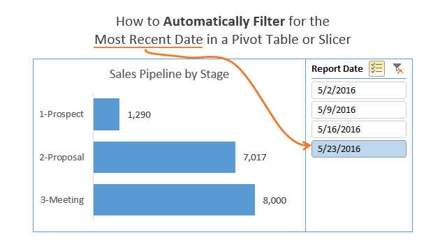
Pip has a set of pivot table based reports that she updates frequently (daily, weekly, monthly).  She wants to automatically filter the reports for the most recent date in a column in the data set.  This filter will select an item in the slicer to filter the pivot tables and charts.

Like everything with Excel, there are a few ways to solve this problem.  We can use a macro, or add a calculated column to the data set…

Download the Example Files

The Setup: CRM Sales Pipeline Data

In this example we are going to use sales pipeline data.  The data table contains weekly snapshots or exports of the data from the CRM system (Salesforces.com, Dynamics CRM, HubSpot, etc.).

To update the data we export a pipeline report every week, and paste the data to the bottom of the existing table.  There are other ways to automate this process, but we won't go into that here.

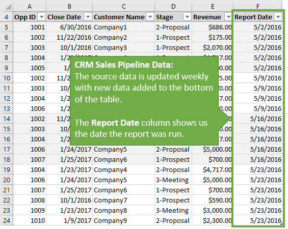
The data set has a “Report Date” column that contains the date the report was run for each row.  You can see in the image that there are 4 sets of data appended (stacked) together to make one large table.

The pivot table shows a summary of revenue by pipeline stage, and there the Report Date field is in the Filters area.  This allows us to filter on any report date to see the pipeline summary for that week.

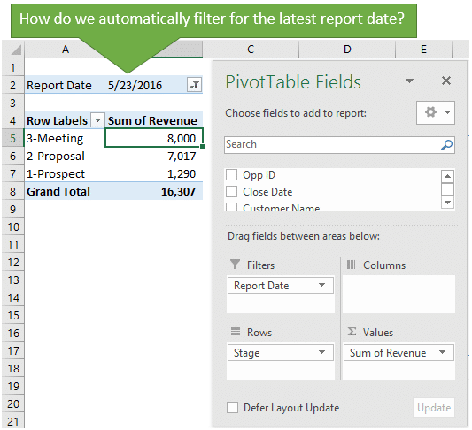
When new data is added to the data table, we want to automatically filter all the connected pivot tables, charts, and slicers for the latest report date.

Solution #1: VBA Macro to Filter a Pivot Table for a Specific Date or Period

We can use a simple macro to set the filter in the pivot table for the latest date in the source data table.  Filtering the Report Date field in the pivot table will also select the filtered item in the slicer, and filter any connected pivot charts.

The macro below might look like a lot of code, but it is actually really simple.  To use it, you will just need to specify all the variables for the worksheet name, pivot table name, pivot field name (Report Date), and filter criteria (latest date).  These variables will represent the names of the objects in your own workbook.

If the macros look like a jumbled mess in you email client, click here to view in your browser.

Sub Filter_PivotField()
'Description: Filter a pivot table or slicer for a specific date or period
'Source: excelcampus.com/vba/filter-pivot-table-slicer-recent-date-period

Dim sSheetName As String
Dim sPivotName As String
Dim sFieldName As String
Dim sFilterCrit As String
Dim pi As PivotItem

    'Set the variables
    sSheetName = "Pivot"
    sPivotName = "PivotTable1"
    sFieldName = "Report Date"
    'sFilterCrit = "5/2/2016"
    sFilterCrit = ThisWorkbook.Worksheets("Data").Range("G2").Value
    
    With ThisWorkbook.Worksheets(sSheetName).PivotTables(sPivotName).PivotFields(sFieldName)
        'Clear all filter of the pivotfield
        .ClearAllFilters
        
        'Loop through pivot items of the pivot field
        'Hide or filter out items that do not match the criteria
        For Each pi In .PivotItems
            If pi.Name <> sFilterCrit Then
                pi.Visible = False
            End If
        Next pi
        
    End With

End Sub

The macro is currently setup to use a value from cell G2 on the Data sheet for the filter criteria (latest date).  Cell G2 contains a formula that returns the latest date from the column using the MAX function.

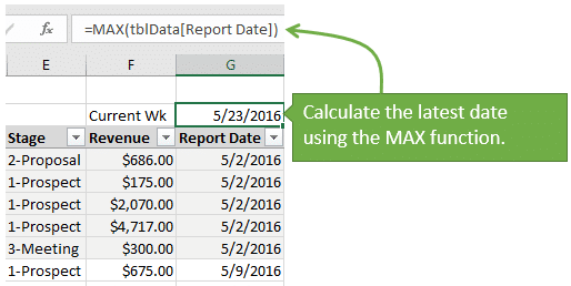
Of course, this could be changed to calculate the latest date in the macro code.  It's nice to be able to see it on the sheet though.

How does the macro work?

The macro first clears all the filters for the Report Filter pivot field with the ClearAllFilters method.

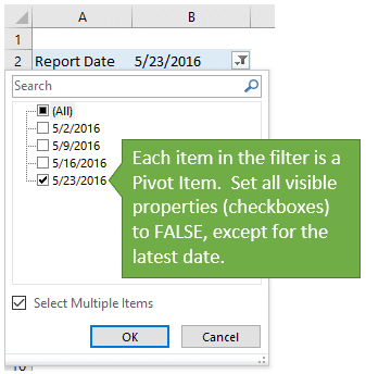
It then uses a For Next loop to loop through all the pivot items in the pivot field to apply the filter.  Each unique item in the field is a pivot item.  The macro checks to see if the pivot item name is NOT equal to (<>) the criteria.  If not, then it hides the item, or filters it out.  That leaves us with only the filter criteria being visible.

I have an article that explains For Next Loops in more detail.

What about filtering two pivot tables for different time periods?

Here is another example with the variables setup as parameters of the macro.  This allows us to call the macro from another macro.

Sub Filter_PivotField_Args( _
    sSheetName As String, _
    sPivotName As String, _
    sFieldName As String, _
    sFilterCrit As String)
'Filter a pivot table or slicer for a specific date or period

Dim pi As PivotItem
    
    With ThisWorkbook.Worksheets(sSheetName).PivotTables(sPivotName).PivotFields(sFieldName)
        'Clear all filter of the pivotfield
        .ClearAllFilters
        
        'Loop through pivot items of the pivot field
        'Hide or filter out items that do not match the criteria
        For Each pi In .PivotItems
            If pi.Name <> sFilterCrit Then
                pi.Visible = False
            End If
        Next pi
    End With

End Sub

Sub Filter_Multiple_Pivots()
'Call the Filter Pivot macro on multiple pivots

Dim sFilter1 As String
Dim sFilter2 As String

    'Set the filter criteria
    sFilter1 = ThisWorkbook.Worksheets("Data").Range("G2").Value
    sFilter2 = ThisWorkbook.Worksheets("Data").Range("G3").Value

    'Call the filter pivot macro to filter both pivots
    Call Filter_PivotField_Args("2 Pivots", "PivotTable1", "Report Date", sFilter1)
    Call Filter_PivotField_Args("2 Pivots", "PivotTable2", "Report Date", sFilter2)

End Sub

In this example we have a sheet with two pivot tables for a week-over-week comparison.  So we need to filter one pivot table for the most current date, and one for the prior week's date.

The Filter_Multiple_Pivots macro calls the Filter_PivotField_Args macro twice.  Notice that the pivot table name and filter criteria values are different for each call.  This is an easy way to reuse the filter pivotfield macro multiple times without having to repeat a lot of code.

Checkout my free video series on getting started with Macros & VBA to learn more about writing macros.

Solution #2: Add a Calculated Column to the Data Set

If you can't use macros then you can solve this problem with a calculated column.  This solution is NOT as flexible as the macro.  It does NOT really work well if you want to have slicers where the user can select other report dates.

We can add a column to the source data to check if the report date in each row is equal the most recent date.  We will call this column “Current Wk”.

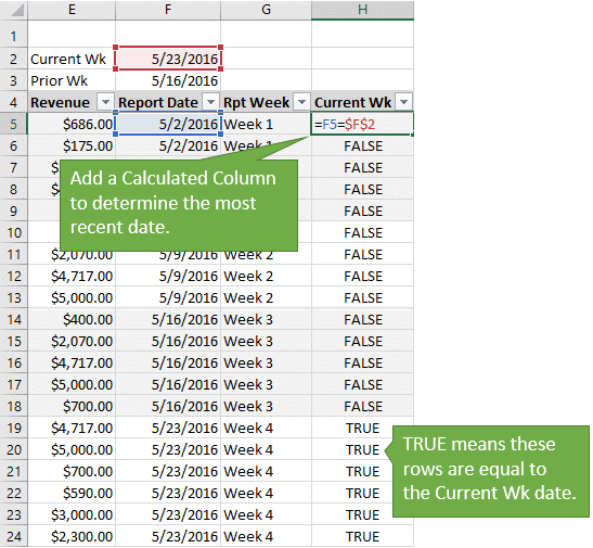
If it is then the formula will return a TRUE, if not it will return a FALSE.

This is a very simple formula.  We could use an If function, but it is not necessary here.  The equal sign will evaluate the match and return a TRUE or FALSE.  Checkout my article on If Statements in Excel formulas for an explanation on this.

We can now add this new column to the Filters area of the pivot table, and filter it for TRUE.  This means that anytime the source data is updated with new data, the formulas will recalculate the new current week rows.  Refreshing the pivot table will automatically apply the filter for the current week rows, and display those in the pivot table.

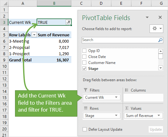
The drawback here is that the user cannot really use a slicer to filter for other dates.  Technically they can, but we will have to reapply the Current Wk filter next time the data is updated.  We could use a macro to automate this, but then we are really back to solution #1.

Although it's not as dynamic as solution #1, the calculated column might be all you need to display the most recent period's data in a static report.

Two Ways to Automate Pivot Table Filtering

Filtering pivot tables for the most current date or period is definitely a good process to automate if you do this task frequently.  This can save us a lot of time, and prevent errors that usually occur with these boring repetitive tasks. 🙂

Please leave a comment below with any questions or suggestions.  Thanks!