Create Multiple Pivot Table Reports with Show Report Filter Pages

Bottom line: Learn how to quickly create multiple pivot table reports with the Show Report Filter Pages feature.  Video tutorial below.

Skill level: Beginner

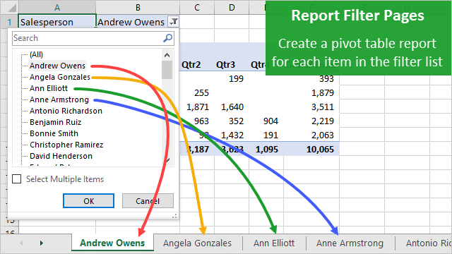
Video: How to Create Multiple Pivot Table Reports Based on a List

Download the File

Download the example Excel file to follow along.

Create a Pivot Table for Each Item in a List

Pivot tables are an amazing tool for quickly summarizing data in Excel.  They save us a TON of time with our everyday work.  There is one “hidden” feature of pivot tables that can save us even more time.

Sometimes we need to replicate a pivot table for each unique item in a field.  This could be a report for each:

• Department in organization.
• Salesperson on the sales team.
• Account in the general ledger.
• Customer in the CRM system.
• Stock in the portfolio.
• Or, just about any other field (column) in your data set.

We could create one pivot table, filter it for a specific item, then copy the sheet and re-apply a filter for the next item.  This would take A LOT of time if we have dozens or hundreds of unique items in the data set.

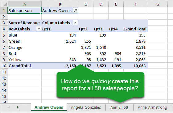
Fortunately, we don't have to do all this manual work.  Pivot tables have a feature called Show Report Filter Pages that automates this entire process.

The Show Report Filter Pages Feature

The Show Report Filter Pages feature:

1. Creates a copy of an existing pivot table for each unique item in a field.
2. The new pivot tables are created on individual worksheets.
3. Each sheet is renamed to match the item name.
4. A filter is applied to the field in the Filters Area of each pivot table for the item.

All this is done with a click of a button.  Your field can have 5 or 500 unique items.  Show Report Filter Pages will create a sheet for each item and replicate the pivot table report.

Here are the steps to use Show Report Filter Pages:

Step 1 – Add the field to the Filters Area

The first step is to create a pivot table.  Then add the field that contains the list of items to the Filters Area of the pivot table.

In this example we want to create one pivot table for each salesperson in the organization.  So, we are going to add the Salesperson field to the Filters Area of the pivot table.

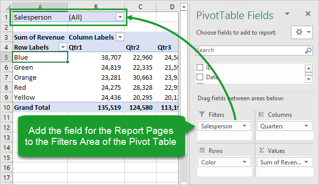
This allows us to filter the entire pivot table for a single sales person.

Check out my videos series on pivot tables and dashboards for more on how to use pivot tables.  I also have a article on how pivot tables work that explains the Filters Area in detail.

Step 2 – Run the Show Report Filter Pages

Once we have the pivot table all setup with the report we want to replicate, we just have to click the Show Report Filter Pages button.

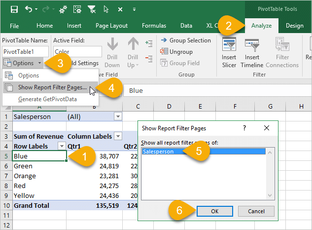
1. Select any cell inside the pivot table.
2. Select the Options/Analyze contextual ribbon tab.
3. Click the drop-down arrow to the right of the Options button on the left side.
4. Click the Show Report Filter Pages… button.
5. The Show Report Filter Pages window will appear with a list of all the fields in the Filter Area of the pivot table.  Select the field to create the reports on
6. Then press OK.
7. Result: A worksheet will be created for each item in the list with a pivot table that is filtered for that item.  The worksheet will also be renamed to match the item name.

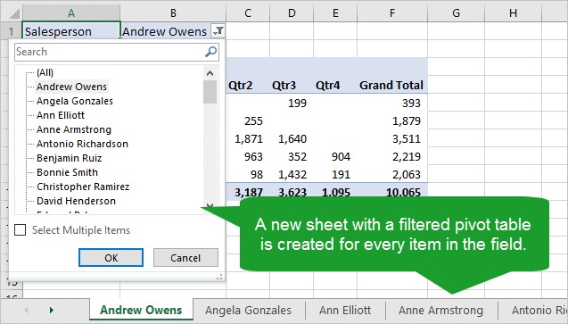
With just a few clicks we have a report for each item in the list.  This can be a huge time saver!

Important Things to Note

There are a few important things to know about Show Report Filter Pages.

Pivot Table Changes are NOT Linked

When we make changes to the original pivot table, those changes will NOT be reflected in the new filter pages pivot tables.  If we wanted to change the layout or formatting of all the reports, it would be best to delete all the filter pages (new worksheets) and generate the reports again.

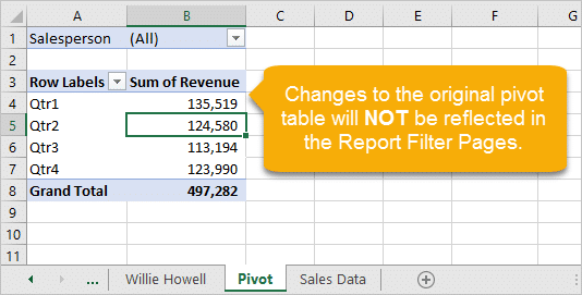
Fortunately, this is pretty easy to do.  We can select multiple sheets by holding the Shift key, then right-click>Delete to delete all the sheets at one time.

Check out my video series on productivity tips for working with sheets for more tips & tricks.

Existing Filters are Applied When Creating Filter Pages

Any filters that are applied to other fields in the pivot table will be applied to all of the new pivot tables.  So, it's best to clear the filters from other fields in the Filters, Rows, or Columns area BEFORE running Show Report Filter Pages.

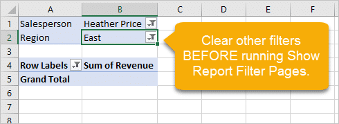
We can also use this to our advantage if we do want to apply filters to all of the reports.  Either way, it's just good to know how this works.  If you generate reports and some of them are blank, it might be due to a filter that is applied somewhere.

Only the Pivot Table is Replicated

Show Report Filter Pages only replicates the pivot table that we run it on.  It is NOT creating a copy of the existing sheet.  It is creating a new sheet and creating the pivot table on a new blank sheet.

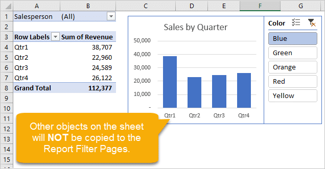
If you have any other formulas, slicers, or charts on the original pivot table sheet, those objects will NOT be copied to the new sheets.  We would need to use a macro to do that type of replication.

Navigate Sheets with The Tab Hound Add-in

At the end of the video I showed how we can use the Tab Hound Add-in to quickly search for any sheet in the workbook, and navigate right to it.  I developed the Tab Hound Add-in specifically for this task of navigating large workbooks that contain a lot of sheets.

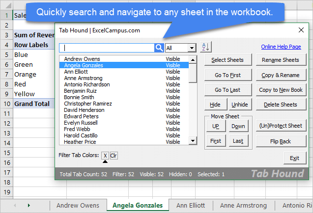
Tab Hound eliminates the horizontal scrolling we typically do to find a sheet in a large workbook.  Instead, you can simply type a search for a sheet name in the Tab Hound window, and jump right to it.

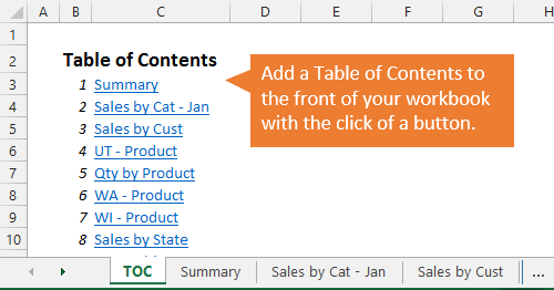
I also shared the Table of Contents feature that allows you to create a Table of Contents with clickable links to each sheet in the workbook.  This will make it easy for your users to navigate these large workbooks that contain a lot of sheets.

Click here to learn more about Tab Hound

What will you use this technique for?  Please leave a comment below with any suggestions or questions.  Thank you! 🙂