3 Ways to Display (Multiple Items) Filter Criteria in a Pivot Table

Bottom line: Learn how to create a list of the (Multiple Items) that are filtered for in the pivot table Fields area.

Skill level: Beginner

Video: 3 Ways to Display (Multiple Items) Filter Criteria

Download File

Download the sample Excel file to follow along.

The (Multiple Items) Dilemma

The Filters area of the pivot table allows us to apply a filter to the entire pivot table.  This is a great way to filter the report to only see data for certain time periods, categories, regions, etc.

We can check the Select Multiple Items box in the filter drop down menu to filter the pivot table for multiple items in the field.  This is a really powerful feature.

However, when we filter for more than one item, the cell that contains the filter drop-down menu displays the phrase “(Multiple Items)”.  There is no way to see what items the pivot table is being filtered for unless we open the filter drop-down menu and scroll through the list.

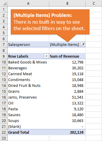
This is time consuming, and can also cause confusion for readers and users of our Excel files.

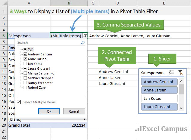
3 Ways to Display the Filter Criteria on the Worksheet

Even though there is no built-in way to display the filter list, I have 3 simple workarounds that can be implemented pretty quickly.

It's important to note that these solutions are additive.  That means in order for solution #3 to work, we will need to implement solutions #1 and #2 first.  Read on and you will see what I mean.

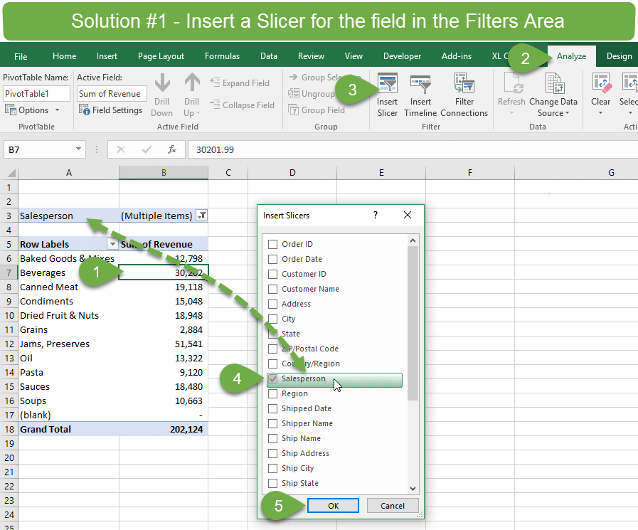
Solution #1 – Add a Slicer to the Pivot Table

The quickest way to see a list of the Multiple Items in the filter is to add a slicer to the pivot table.

1. Select any cell in the pivot table.
2. Select the Analyze/Options tab in the ribbon.
3. Click the Insert Slicer button.
4. Check the box for the field that is in the Filters area with the filter applied to it.
5. Press OK.

A slicer will be added to the worksheet.  The items that are selected in the filter drop-down list will also be selected/highlighted in the slicer.  These two controls work interchangeably, and we can use both the slicer and the filter drop-down menu to apply filters to the pivot table.

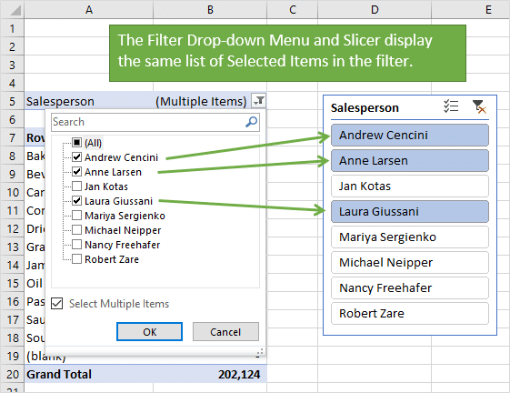
The slicer is a great solution if you only have a few items in the filter list.  If you have dozens or hundreds of items in the filter list, then the user is required to scroll horizontally through the slicer to see the selected items.  So, it's not the best solution for long filter lists.

Solution #2 – Add a Connected Pivot Table

We can list out all of the selected filter items in cells on the worksheet with another pivot table.  Here is a quick guide of the steps to create the connected pivot table.  Please watch the video above for further instructions.

It's important to note that we still need the slicer created in Solution #1 for this to work.

1. Select the entire pivot table.
2. Copy and paste it to a blank area in the worksheet.
3. In the new pivot table, move the field in the Filters area to the Rows area.
4. Remove all other fields in the pivot table so there is only one field in the Rows area.
5. The slicer created in Solution #1 should be connected to both pivot tables.  If not, right-click the slicer > Report/Pivot Table Connections, and check the boxes for both pivot tables on this sheet.

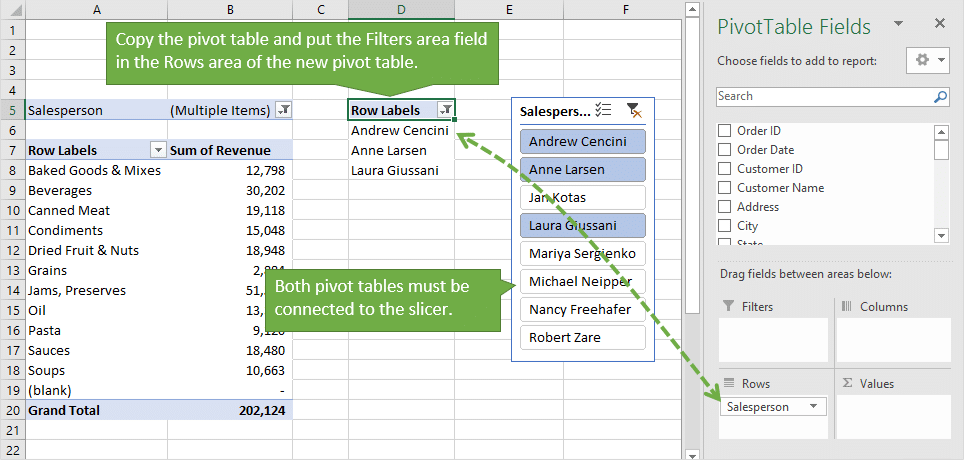
This new pivot table will display a list of the items that are filtered for in the first pivot table.  As filters are applied to the Filters area of the first pivot table, the second pivot table automatically updates to display the filter items.  This happens because both pivot tables are connected by the slicer.  Pretty cool stuff! 🙂

This solution allows us to create formulas based on the list of applied filter items in the pivot table.  We can use this in all types of scenarios for creating interactive reports, dashboards and financial models.  The possibilities are endless.  Solution #3 is an example of how to use the results in a formula.

Solution #3 – Create a Comma Separated List of Filter Items

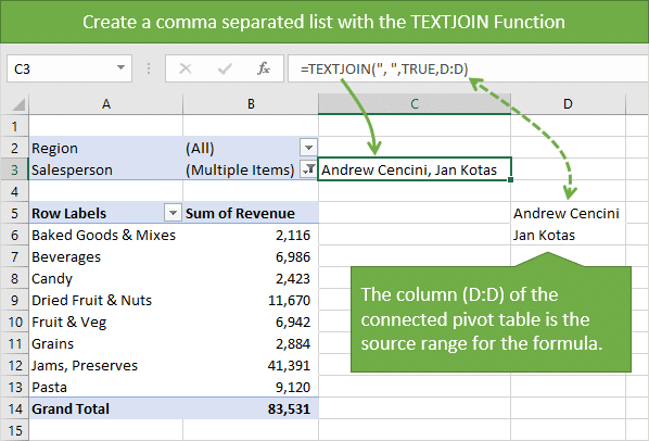
The list of filter items can also be joined into one list of comma separated values in one cell.  This is nice if you want to display the list right next to the pivot table.

We can easily create this list with the new TEXTJOIN function that was introduced in Excel 2016.  If you don't have Excel 2016 or Office 365 yet, then you can also do this with the CONCATENATE function.  It's just more work to setup.

Again, for this to work we will need to implement solutions #1 and #2 first.  Here are the steps.  Checkout the video above for more details.

1. Type =TEXTJOIN( in the cell where you want to display the list.
2. TEXTJOIN has 3 arguments.  The first argument is the delimiter or separator between each cell value.  We can put just about anything we want in here.  We just have to wrap the delimiter in quotation marks.  To separate the values with commas, put a comma followed by a space in the argument: “, ”  Then type a comma.
3. The 2nd argument is the ignore_empty option.  This allows us to ignore empty cells and requires a TRUE/FALSE value.  We will select TRUE to ignore any empty cells.  That means empty cells will not be added to our list.
4. The 3rd argument is the text.  For this argument we can reference a range of cells.  In this case we will reference the entire column of the second pivot table in Solution #2.  Since the TEXTJOIN function is going to ignore empty cells, we can reference the entire column.  The filter list will grow/shrink depending on how many filter items are selected.  This makes the output of TEXTJOIN dynamic, without having to create a dynamic named range.
5. Close the parenthesis on the formula and hit Enter to see the results.
6. The list will also contain the header label of the Rows area of the pivot table.  We can remove this by turning off the Field Headers.  This is a toggle button on the Analyze/Options tab of the ribbon in the Show section.

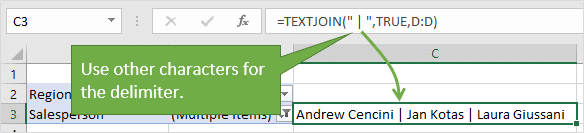
There are a lot of options with this solution.  We can change the delimiter to a different character besides a comma.  We can even use the line break character CHAR(10) to list each item on a new line in the same cell.  Just apply Wrap Text to the cell.

Another option for the delimiter is the pipe character. ” | “

What if I don't have TEXTJOIN?

If you aren't using Excel 2016 or Office 365 yet, then you can create this formula with the CONCATENATE function.  It is just more work to setup.  However, I have a free macro that creates the CONCATENATE formula for you, including the delimiter character.

Multiple Ways to List Multiple Items

Well, there are 3 ways to list and display the filter items on the worksheet.  The magic here is in the slicer that allows us to create connections between pivot tables.  Checkout my article on how slicers and pivot tables are connected for a detail explanation on this relationship.  I also have a video on how to use slicers.  You can share this with your co-workers and users that are not familiar with using slicers.

I also have a free 3-part video series on Filters in Excel that is part of my Filters 101 Course.

My free 3-part video series on pivot tables and dashboards explains more about creating interactive reports with slicers and charts.

Please leave a comment below with any questions.  I'm interested to hear how you will implement these techniques in your Excel files.  Thank you! 🙂