Bottom line: Learn how to get the pivot table to default to a Sum calculation instead of Count when the source data field contains numbers.
Skill level: Beginner
Video: How to Default the Pivot Table Calculation Type to Sum
Watch in full screen HD or on Youtube.
Why does the Pivot Table Default to Count?
One of the most common questions I see on my free 3-part video series on pivot tables & dashboards is, “Why does the pivot table default to Count instead of Sum when I add a field to the values area?”
Well, Pivot Tables have some rules on which calculation type will be selected when we add a field to the Values area.
The rules are pretty simple:
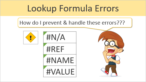
- If ANY cell in the column (field) contains text, blanks, or errors (#N/A, #REF!, #VALUE!, #NAME?), then the calculation type will default to COUNT.
- If ALL cells in the column (field) contain numbers, then the calculation type will default to SUM.
Now that we know the rules, we can prevent this error by cleaning up our data.
How to Prevent the Default Count Calculation Type
Let's take a look at 3 ways to make sure the calculation type defaults to Sum.
1. Replace Blank Cells with Zeros
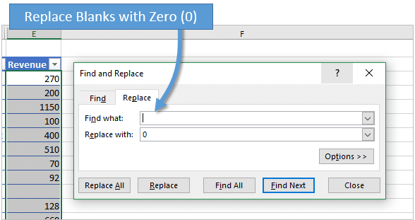
In the video above I show a data set that contains blanks in the Revenue column. Since there are blanks in this column, the pivot table calculation type defaults to Count.
One quick way to fix this is to replace the blank cells with a zero (0) value. Here are instructions on how to find & replace all blanks in a column.
- Select all cells in the column or Table (keyboard shortcut: Ctrl+Space Bar).
- Open the Replace Window from the Home tab on the Ribbon in the Find & Select menu (keyboard shortcut: Ctrl+H).
- Delete everything in the Find What text box so it finds blank cells.
- Type a zero 0 in the Replace With box.
- Press the Replace All button (keyboard shortcut: Alt+A).
- Refresh the pivot table (keyboard shortcut: Alt+F5).
- Add the field to the Values area of the pivot table.
The calculation type should default to a Sum calculation if all cells in the data source column are numbers.
2. Replace Errors with Zeros
Blank cells are the most common cause that I see for calculation type defaulting to Count. However, cells that contain text or errors can also cause this problem.
If the source data column contains a formula that is returning errors, we can use an IFERROR function to return a zero instead of the error. Of course we will want to determine why the error is occurring in the first place.
My free 3-part video series on the lookup formulas has an entire video dedicated to learning how to prevent and fix errors with formulas like VLOOKUP and INDEX/MATCH.
3. Convert Text to Numbers
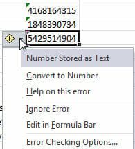
Sometimes values in cells look like numbers, but the numbers are stored as text. This is a common issue when you are importing data into Excel from another system. In this case we will need to convert the text to numbers first. Checkout my article on keyboard shortcuts to convert text to numbers to learn more about these techniques.
PivotPal's Auto Sum/Count Feature
At the end of the video I also explain how PivotPal can save time with this issue. PivotPal has it's own rules for adding a field to the values area, and does NOT default to count if the column contains blanks.
If the column contains numbers and blanks, PivotPal will default the calculation type to Sum when we add the field to the values area using the PivotPal window. This is one way to get around this annoying issue without having to modify the source data.
The PivotPal Add-in is packed with features that will save you time when working with pivot tables in Excel. Please click the link below to learn more and give PivotPal a try today.
Click here to learn more about The PivotPal Add-in
Free Webinar on Pivot Tables
Right now my good friend John Michaloudis from My Excel Online has a pivot table webinar going on. This is a free hour long training on how to get started with pivot tables in Excel.
Here are some of the Excel skills you will learn:
- How to set up your data and create a Pivot Table in less than 3 minutes which will increase your efficiency!
- How to put your key business metrics like Year to Date Sales, Monthly Variations and Top 10 Customers in an interactive Pivot Table, taking your analytical skills to another level;
- How to create an Interactive Dashboard with Slicers & Pivot Charts that will WOW your boss and get you noticed by top Management;
- Pivot Table tips & special Bonus attendee material that you can keep and use to become better at Excel straight away which will skyrocket your personal development!
Click the link below to register for the free webinar and pick a time that works for you.
Click here to register for the free webinar on pivot tables
What Other Issues Cause the Calculation to Default to Count?
Is your calculation type still defaulting to Count? This is typically due to one or more cells that are NOT numbers. Please leave a comment below with any other issues that I might have missed, or any questions you have. Thank you! 🙂


Jon,
Thank you for sharing your knowledge regarding excel – very helpful and greatly appreciated. I have a question for you:
I am seeking to clean up my CRM data base which includes approximately 9,000 company names. I have exported the data into an excel file so I can quickly identify various issues. I want to identify and eliminate duplicates and near duplicate entries. I have used the duplicate function within the Conditional Formatting function and it has color coded various duplicates. However, it only identifies exact text duplicates, which is understandable and valuable. I would like to use a Fuzzy Logic Duplicate Finder function to find near approximates for entries which are similar, yet different only by a character, a period or coma or abbreviation. I saw that this function is available for the Windows version of excel 2016. I am using a mac and have the 2016 version of excel. Can you provide me with guidance on how I can locate near duplicate – with with an established function or through a series of steps? Many thanks, Brian Kerester
Hi Brian,
Thanks for nice feedback! I don’t know of an add-in for the Mac that does this. However, there is a fuzzy match add-on for Google Sheets. I have not tried it, but might be worth a shot. I hope that helps.
This is useful. I had this problem a few weeks ago. Eventually, I identified the issues as having to do with blank cells, but didn’t go about fixing it.
Thank you Dan!
Another Excel annoyance explained … thanks. I don’t know if you have covered this topic before, but tips on cleaning up a pivot table – e.g. formatting, fixing column width, etc. – would be helpful.
Thanks Tom! I will add that to the list. 🙂
Dear Jon,
All of your videos that I have watch are very informative and easy to understand. You are really doing great service to all Excel users.
Thank you Asif. I really appreciate that. 🙂
Hi Jon,
This article is a very helpful and well-assembled tutorial on solving this most intractable and irksome of pivot table issues that often pops up several hours in to assembling a complex report. Thank you very much for collecting and arraying all of this info in one single very useful source, most appreciated!
Thanks Ian! I’m happy to hear you found it useful. Excel has a lot of little quirks like this that can be somewhat of a mystery sometimes.
thank you so much you helped me to save a huge problem 🙂
My pivot changes to zero every time i want to change it to sum from count
I am having the same problem. Did you find out how to get it to SUM?
I found my problem. Turns out the incoming data for this specific field was formatted as TEXT. I converted it to NUMERIC, then the pivot table SUM worked fine.
Pivot table defaulting to Count not Sum. All values are numbers, no errors, no blanks in the data
Thank you for solving the default calc type in pivots. has always puzzled me; but makes sense.
Thank you very much for detailed understanding.
Thank you for the tutorial. I have further question, I have a data that looks like this “$100B” which stands obviously for 100 Billioon dollars. Excel reads it as text because of the “B”. I have tried to change to a number using the “column to text” function. I did not work. There are no blank spaces or erros. I also tried to cut it using the “Right and Left” function but the data have different ranges from 100B to 1B. Trimming is not also a good option. What is the best and reliable solution? Thank you
Jon thank you so much for your help! You have no idea how much appreciation I have for your explanation.
Hope you are doing great.