How To Compare Multiple Lists of Names with a Pivot Table

In this post I will explain how to compare two or more lists of names using a Pivot Table.

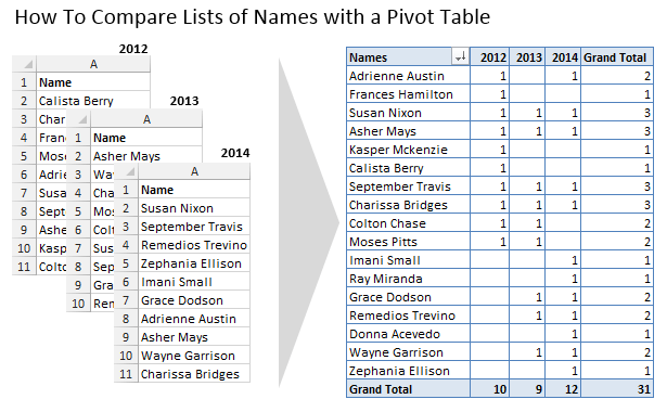
In this example we have lists of names for people that signed up to volunteer for a beach cleanup event.  The event has been running for three years and we have one list for each of the last three years.

We want to compare these lists and answer some of the following questions about our volunteers.

• Who has signed up all three years?
• Who signed up last year, but did not sign up this year?
• Who is new to the event this year?

Video

The Pivot Table List Comparison Technique

We can answer all of these questions with one very simple Pivot Table.  This technique is very easy to implement and does not require any formulas.

It should also help you understand how Pivot Tables work to consolidate and summarize data.

In three simple steps we are going to create the pivot table and answer our questions.

You can download the sample file I'm using to follow along.

Don't forget to sign-up for my free email newsletter to get more tips and downloads like this.

Step #1 – Combine the Lists

The first step is to prepare our lists.  In the file we have three worksheets that contain a list of names for volunteers that signed up each year.

We need to combine these three lists into one list that contains all the data for all three years.

The following are the steps for combining the lists.

1. Make a copy of the ‘2012' sheet and rename it to ‘Combined Data'.
2. In cell E1 add the text “Year”.  This new column will represent the year for each list of data.
3. Enter “2012” in cell B2 and copy it down to the end of the list.
4. Copy the 2013 data to the bottom of the list on the ‘Combined Data' sheet.
5. Enter “2013” in column B in the first row of the 2013 data (cell B12), and copy it down to the end of the list.
6. Repeat steps 4 & 5 for the 2014 data.

You should now have a long list of data that contains all the data rows for all three years, with a new column (B) that specifies which year the data row belongs to.

Please see my article on structuring source data for pivot tables for detailed explanation on why the data is organized like this.

Step #2 – Create the Pivot Table

We can now create a Pivot Table based on our ‘Combined Data' list to start making comparisons.

Here are the steps to creating the Pivot Table.

1. Select a cell in the Combined List and press the Pivot Table button on the Insert tab of the Ribbon.  Press OK on the prompt window to create a Pivot Table on a new worksheet.
2. Add the Name field to the Rows area of the Pivot Table.
3. Add the Year field to the Columns area of the Pivot Table.
4. Add the Name field to the Values area of the Pivot Table.  This will create a Count of Names measure.

You should now have a list of names of all the volunteers that signed up over the last three years.  The “1's” in columns B:D tell us that the person was a volunteer in that year.

The Pivot Table Explained

When we add the Name field to the Rows area of the pivot table (step 2 above), Excel automatically consolidates the list for us and creates a row for each unique name from the combined list.  This means that names that appear in multiple years will only be listed once.

For example, the name Asher Mays appears three times in the combined list (source data of the pivot table).  But the pivot table only displays the name once in row 6 (image below).  This is a consolidated list of unique values.

The same thing happens when we add the Years field to the Columns area (step 3 above).  The years 2012, 2013, and 2014 are listed many times in column B of the combined data list.  But each of the years only appears once in columns B:D of the pivot table.

When we add the Names field to the Values area (step 4 above), Excel calculates how many times the name and year combination appear for each intersection in the pivot table.  For example, cell C6 of the pivot table is the intersection of the name Asher Mays and the year 2013.  This combination appears once in the data source, so a “1” is displayed in cell C6.

If a cell in the pivot table is blank then that name and year combination does not exist in the source data.  That means the person did not volunteer that year.

Step #3 – Answer Our Questions (Analyze the Results)

We can now use this one Pivot Table to answer all of our questions.

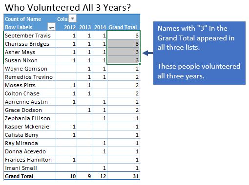
Question #1 – Who has signed up all three years?

Column E of the Pivot Table contains the Grand Total (sum of columns B:D).   People that volunteered all three years will have a “3” in column E.

We should sort the pivot table so all the people with a “3” in column E appear at the top of the list.  This will make it easier to find the names.

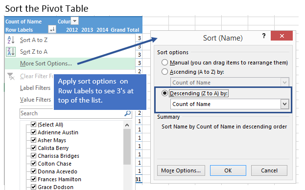
These people will have a “1” in each column from B:D and the sum of these 1's = 3.

If your list is longer, you can copy the Pivot Table data to another sheet and use Excel's Filter features to sort and filter the data further.  You can also use an Excel Table to automatically summarize your filtered results.  Checkout my video on Excel Tables to learn about tables.

Question #2 – Who signed up last year, but did not sign up this year?

To answer this question we need to know who had a “1” in the 2013 column and a “blank” in the 2014 column.

The filter features of the Pivot Table can be somewhat limited for this exercise, so I will copy and paste the pivot table data to another sheet and apply Filters to do the analysis.

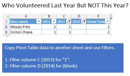
These are people we might want to contact to see if they can make it this year.

Question #3 – Who is new to the event this year?

To answer this question we just need to know who has a “1” in the 2014 column, and blanks for 2012 and 2013.

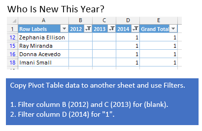
This tells us that the person has never volunteered before, and we want to be extra nice to them so they come back next year. 🙂

Checkout my article on 7 Keyboard Shortcuts for the Drop-down Filters for some quick tips on using the Filters.

What's Next?

This technique to compare multiple lists of data using a Pivot Table is “must-know” for any analyst.  It is very easy once you get the hang of it, and it will save you a lot of time.

The alternative is to use a lot of VLOOKUP, SUMIF, or COUNTIF formulas, and you will spend a lot of time manually creating a report.

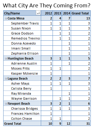
The Pivot Table technique can also let you quickly pivot to answer other questions about your data.  For example, if we wanted to know what city our volunteers are coming from, we could easily add the City field to the Rows area of the Pivot Table.

This allows us to further analyze our data  and see that we might be continually attracting volunteers from some cities and not others.

I've really just scratched the surface of how you can use this technique.

In an upcoming post I will show you how you can use this same technique to reconcile transaction data.  Do you have a list of accounts or customer (CRM) data, where you want to see what changed from last month to this month?

I will show you how to use this technique to create some very powerful reports that will give you a lot of insight into your data.

Please subscribe below to get an email when this new post is available.  And leave a comment below with any questions. 🙂