Bottom line: Learn how to add total rows and columns to the bottom of the spill ranges created by dynamic array formulas.
Skill level: Advanced
Video Tutorial
Download the Excel File
You can download the example file I use in the video below to follow along.
Floating Totals for Spill Ranges?
Thomas, a member of our Elevate Excel Training Program, asked a great question in the Community Forum about adding total rows or summary rows to spill ranges.
This is NOT directly possible in Excel yet. However, I recently stumbled upon an interesting range reference that allows us to create a workaround solution.
The solution just uses a few Dynamic Array formulas and Conditional Formatting. I can't say it's easy, but I think the technique will be very useful in many different scenarios.
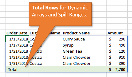
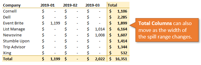
The Problem: Spill Ranges Change Size
Dynamic array formulas are an awesome way to create interactive summary reports, and can be used as an alternative to pivot tables. The spill ranges will typically change size (more or less rows or columns) as input values change.
One common issue with dynamic arrays is that we can't append data to the bottom of the spill ranges yet.
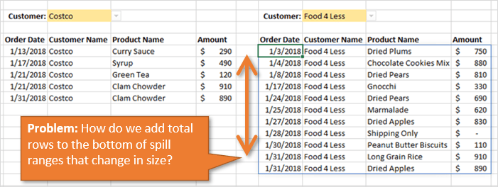
In the example above I'm using the FILTER function to create a report by customer. The number of rows in the spill range changes when a new selection is made from the Customer drop-down list.
Therefore, it's difficult to put a total row below the spill range because the last row of the spill range is constantly changing.
If you're not familiar with dynamic arrays yet, then checkout my post & video on Dynamic Array Formulas and Spill Ranges. You will also want to make sure you are on a version of Excel that has dynamic arrays.
The Solution: The Overflowing Spill Range?
So, we need a way to append total rows or columns to the bottom of the spill range, and/or include them inside the spill range.
One possible solution uses this weird range reference:
=G7#:G6
It allows us to use the spill range operator and create a range reference that includes rows and columns ABOVE and to the LEFT of the spill range.
I'm not sure if there is a term for this yet, but I'm calling it an overflowing spill range. 🙂
This means we can put our total rows/columns above or to the left of a spill range, then use the SORTBY function to move them to the bottom/right.
If that sounds crazy, well, buckle up…
Update: A New Solution with VSTACK
In April 2022, Microsoft released the new VSTACK and HSTACK functions (along with 12 other new functions) that make this process easier.
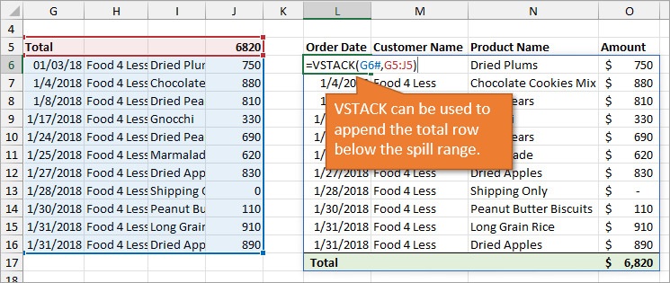
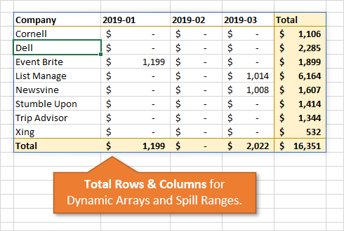
VSTACK allows you to append ranges together into one spill range. In this scenario we can use it to include the total row below a spill range. We can also use HSTACK to put a total column to the right.
This solution allows you to SKIP steps 3 and 4 below. Not everyone has VSTACK yet, so the overflowing spill range solution will still apply. Plus it might be a useful technique in other scenarios.
The Explanation: Total Rows for Spill Ranges
There are two major ingredients for this technique: dynamic array formulas and conditional formatting. The solution does NOT use VBA or macros.
Let's take a look at each component.
Step 1: Write the Formulas
There are four major formula components that go into the solution.
The first three components can be created in a staging/calculation area on a separate worksheet. The fourth component will be the formula that spills the final output with the total rows/columns.
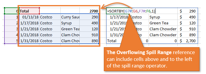
#1 – The Original Spill Range
The first thing we need is a spill range for the summary report. You can use ANY dynamic array formula that produces a spill range.
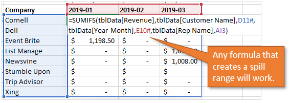
In the example above I used a FILTER function. Here is another example that uses the SUMIFS function to produce a spill range.
#2 – The Total Row
Next we need to create the total row(s) directly above the original spill range.
Type the word Total in the left most cell.
Note: You do NOT have to use the word Total. This can be any phrase. It just needs to be different from any values in the left column of the spill range to differentiate it for the conditional formatting.
Next you'll create the formulas for the total row. You can use any formula to calculate various metrics: sum, average, count, etc.
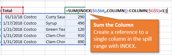
In the first example I use the SUM function to sum individual columns in the original spill range. That formula looks like the following.
=SUM(INDEX($G$6#,,COLUMN()-COLUMN($G$5)+1))
It uses the INDEX function to return a range reference to a single column in the spill range (G6#). See the video above for further explanation.
You can also use a SUMIFS formula here to create a sum from the source data range.
#3 – The Index Column
Note: If you have VSTACK then you can skip this step and step 4. See the section at the beginning of the article for more info.
Next we need a way to put the total row at the bottom. We're going to create an “index column” that contains row numbers. This can be to the left or right of the original spill range, and does not need to be directly next to it.
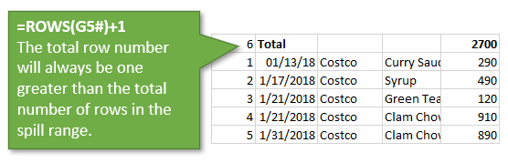
There are two formulas for the index column:
- The SEQUENCE function is used to create row numbers for each row of the spill range. Put the following formula in the same row as the first row of the original spill range and reference it with the spill range operator.
=SEQUENCE(ROWS(G6#))
This creates a list of numbers from 1 to the number of rows in the original spill range. - The row number for the total row is 1 greater than the number of rows in the spill range. Put the following formula next to the cell in the total row.
=ROWS(G6#)+1
This formula counts the number of rows in the spill range and adds 1, ensuring that the total row will always be at the bottom when it's sorted.
#4 – The Sorted Output Range
Finally, we are going to sort the data in a new output range using the SORTBY function. This formula can be on a separate sheet where you are creating your summary report or dashboard.
This formula uses the overflowing spill range reference that I mentioned earlier, and looks like the following:
=SORTBY(G6#:G5,F6#:F5,1)
The first argument is the array or range we want to sort (G6#:G5). For this we only include the original spill range using the spill range operator (G6#) to the row above that contains the total row (G5).
Interestingly, this reference includes all of the cells from G5 to the bottom right corner of the spill range.
Note: If you ever type a reference with a cell above or to the left last in the range (B100:A1), Excel will usually fix it automatically (A1:B100). However, it doesn't fix it in the case of named ranges and spill ranges. Awesome!
The second argument is the by_array or range we want to sort by. For this we reference our index column with the same range reference (F6#:F5). This includes all of the cells in the sequence function (F6#) and the cell above that contains the row number of the total row (F5).
The third argument is the sort_order and we specify 1 for ascending order.
This SORTBY formula allows us to create a spill range with total row(s) at the bottom of a spill range. Now we need to polish it up with some conditional formatting.
Step 2: Apply Conditional Formatting
With all this hard work to create the total row, we now need it to stand out!
Since the position of the total row will likely change, we can't just apply formatting to a single row on the sheet. Conditional formatting to the rescue.
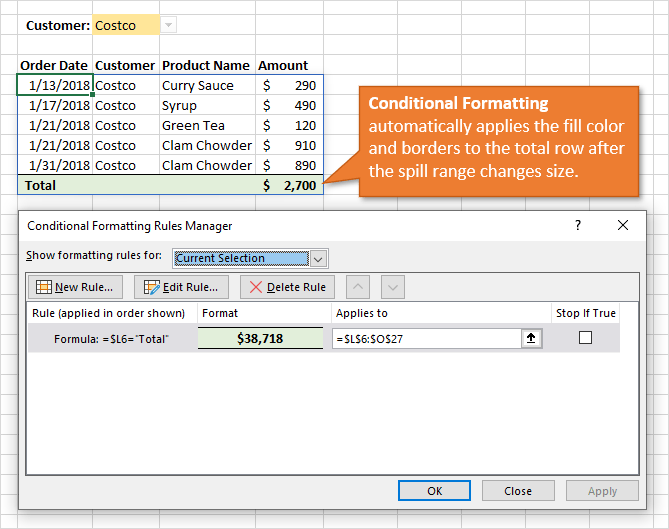
Here are the steps to apply the conditional formatting. See the video above for more details.
- Select a range from the top left corner of the output range (SORTBY formula) to the right-most row and go down the maximum number of rows the range can spill to, plus one for the total row. We can't make the conditional formatting range dynamic yet, so just go down more rows than you will likely need.
- Create a new conditional formatting rule by going to the Home tab > Conditional Formatting > New Rule…
- In the New Formatting Rule window, select Use a formula to determine which cells to format.
- Add a formula that uses a mixed reference for the top left cell in the selection and is equal to the phrase you used for the left cell in the total row.
=$L6=”Total”
Notice that $ symbol in front of the L to make the column an absolute reference and the row number is relative. This applied the formatting to the entire total row where the value in column L equals Total (when the formula evaluates to TRUE). - Click the Format… button to create the formatting for the total row.
- Number tab: See the video on how to hide the zeros in columns that don't contain a calculation. You will use a custom number format and leave the format for the zero blank. The Accounting style custom format looks like the following: ($* #,##0);($* (#,##0);;(@_)
- Font tab: Change the font to Bold, or whatever your preference is. You can also change the font color.
- Border tab: Add a top border and a bottom border if you like. You can also change the color of the border before adding it.
- Fill tab: Select the fill color to make the total row stand out.
- Press OK a few times to apply the formatting to the total row.
If you have multiple total rows you will just repeat this process for the other names used in the left cells of those rows.
The formatting will automatically be applied to the total row(s) as the spill range changes size. If you've made it this far then pause and do the happy dance. It's fun to see it all work! 😀
Additional Uses
There are a lot of uses for this technique and it really all stems from the ability to create a range reference that includes the entire spill range and cells above and to the left of it (the overflowing spill range).
We can add multiple total rows to the bottom by creating total rows with row index numbers that are sequentially greater than the total number of rows in the spill range.
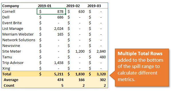
We can also add total columns to the right of the spill range and even have the total column move right/left if the number of columns in the spill range is changing.
See the video above and example file for more on those techniques.
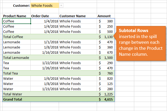
We can also use this technique to add subtotal rows within our spill range. I'll leave that for another post, but it's essentially using multiple total rows and getting the row order correct in the index column.
Alternate Solutions
Another solution is to put the total row way below the spill range and then use the FILTER function to filter out the blank rows between. This solution is a bit less flexible and has the potential for more #SPILL! errors.
You will also need to filter by a column that will NEVER contain blank cells in the spill range. Or you can put a column to the left of the spill range that identifies complete blank rows with the COUNTA function.
You will still use the same technique to conditionally format the total rows in the output range.
If you've been screaming, “why not use a pivot table?!?” as you read this, well you have a point. Pivot tables are a good alternative solution to dynamic arrays. There are pros & cons to each, and I'll leave that as a topic for a separate post.
Conclusion
I can't say this is the easiest solution, but I do believe the overflowing spill range has a lot of potential uses that are yet to be discovered.
So please leave a comment below with any questions, suggestions, or ideas on how we can use this technique to solve other problems.
Thank you! 🙂
Free Training Webinar on the Power Tools
Interested in learning more about the new tools and features of Excel?
Right now I'm running a free training webinar on all of the Power Tools in Excel. This includes Power Query, Power Pivot, Power BI, pivot tables, macros & VBA, and more.
It's called The Modern Excel Blueprint. During the webinar I explain what these tools are and how they can fit into your workflow.

You will also learn how to become the Excel Hero of your organization, that go-to gal or guy that everyone relies on for Excel help and fun projects.
The webinar is running at multiple days and times. Please click the link below to get registered and save your seat.


Thank you, Jon! I was using sumifs on the top portion of the spilled data. I like this alternative. A little steeper learning curve to master, but I love the technique!
This does not address the many uses above, just the ability to create a single formula that brings in data, SPILL-style, and has a Total below the data shown. It is the scratchpad working formula, hardcoded for a useless bit of sample data, but can easily be dressed up to be dynamic in creation of the two ranges in it, with the larger one’s size simply one row greater than the report data’s SPILL size. In the formula, A1:A16 has the source data and J1:J25 is simply sized large enough for me to build the formula, then add data into the source range and see the Total move down as the output range reflects the additions:
=IF(ROW($J$1:$J$25)-1>COUNTA($A$1:$A$16),””,
IF(ROW($A$1:$A$16)<=COUNTA($A$1:$A$16),$A$1:$A$16,
IF(ROW($J$1:$J$25)-1=COUNTA($A$1:$A$16),SUM($A$1:$A$16),
"")))
It reflects whatever data is available, but is not optimized to allow blank rows inside the data set (A7 being blank, say while cells above and below are filled), but that wouldn't be hard either. Any rows in the output range other than the one you choose to hold the Total (if you like a blank row between it and the data, it's just a touch more complicated).
It would work using Table references, but I have read SPILL functionality does NOT work IN Tables, yet, though one could think that would not be an issue since the Table in question would be a data source and not need Totals itself while the output report, which would have the Total, would presumably not be a Table, so…
To be sure, adapting it to provide the SubTotals done in Jon's work would likely be a nightmare, so again, just providing a working concept of "floating totals for spill ranges" as Mr. Kerr asks about. Also, it does not need a helper column (not something I mind, but so many people do).
Of course, the work could be put into Named Ranges or helped in clarity by the new LET() function once people have that. I do like a nice Named Range.
The "overflowing spill range" ranges are a variation on creating ranges like "A1:C3:D2:D3:G1:G5:B2:B7" (what I like to call "calico ranges") and they are resolved the same way by Excel: it does NOT relabel the range (in this case for example, it does NOT replace what I typed with "A1:G7") like it will for a simple range "reversal" like "B100:A1" being replaced with "A1:B100" but it DOES deal with my example as if it were the "full" rectangle that includes ALL the cell pairs refererenced in such a range. Interestingly, it will still only color highlight the exact pairs written, but the output will include all of "A1:G7" including whatever happens due to blank cells in the full rectangle when output wherever you have it. It SUM()'s the entire range, not just the color highlighted cells of the written expression, and so on. (That's the larger point, the smaller being that it Jon's range weren't contiguous, one would have display issues to handle.) Nice though. I'm gonna check next how it can be used if one specifies two SPILL ranges as the calico range.
Many thanks. Very clever work around. I expect future updates will eliminate the need for the middle step.
Here is another approach, no intermediate table needed:
=LET(d,FILTER(tblSales,tblSales[Customer Name]=$M$3),r,ROWS(d),s,SUM(INDEX(d,0,4)),IF(SEQUENCE(r+1)>r,CHOOSE({1,2,3,4},”Total”,””,””,s),d))
Cool, but a lot of work when you can put the totals at the top ;-}
Hi Jon,
Great post, I’d like to think that MS will update the Dynamic Array functionality to include optional totals
Instead of using “=ROWS(G6#)+1” to calculate the index value for the Total row, I’d use 1e9 (my go to BIG number)
My solution to this problem was to simply have the totals at the top, which is often more convenient as it means they’re always in the same position and can be frozen to be always visible (you’ve just got to convince the user that they actually prefer the simpler solution 😉 )
The idea of using SORTBY to drop the Totals row to the bottom was new to me. I had used the rather more prosaic
= LET(
selectedValue, FILTER(value, name=selected),
totalValue, SUM(selectedValue),
count, COUNT(selectedValue),
k, SEQUENCE(1+count),
IF(k<=count, selectedValue, totalValue) )
What may rate as a touch more creative is the conditional format based on the formula
=CF?
where the Boolean 'CF?' is defined to refer to
= LET(
count, COUNT(result#),
finalCell, INDEX(result#, count),
ISREF(currentCell finalCell) )
and the final line is the intersection of the current cell and the final cell of the spilt range.
This was very very useful. Excellent idea on how to solve a problem I have had for a long time.
Please upload your take on doing subtotals on spill ranges, will help me a lot.
Keep it up with your great lessons.
[…] To illustrate this further, I would like to cover a technique discovered by Jon Acampora in this post: https://www.excelcampus.com/functions/total-rows-dynamic-arrays […]
Hello
Is it possible to get example how to add subtotal to spill ranges
Thanks in advance