Bottom Line: With Excel's latest update, you can now create dynamic reports in multiple languages, making your spreadsheets more accessible and user-friendly for international audiences.
Skill Level: Intermediate to Advanced
Watch the Tutorial
Download the Excel File
You can follow along using the Excel files I used in the video.
Getting Started with the Translate Function
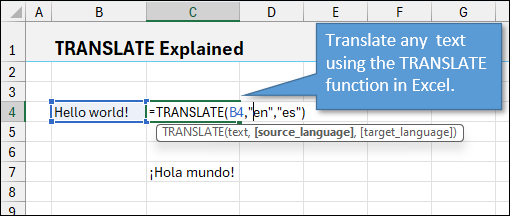
Excel’s TRANSLATE function is a new feature, allowing you to translate text in your reports with ease. Here's how:
- In any cell, type
=TRANSLATE. - Select the text you want to translate (for example, cell B4), choose the source language (for example, “en” for English), and the target language (such as “es” for Spanish).
- Hit Enter and watch your text transform into the selected language.
This function taps into Microsoft’s translation service, and though it's currently in Beta, it's incredibly effective for multilingual reports.
Creating a Dynamic Report with Language Selection
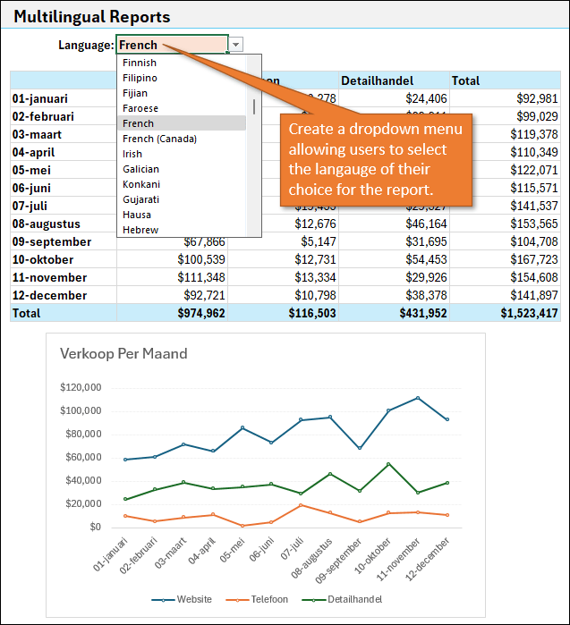
A big part of the magic happens when you allow users to select their desired language via a dropdown menu. Here's how to create that dropdown.
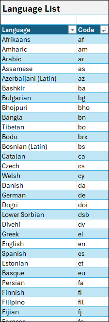
- Prepare Your Language List:
- Create a table or list of languages and their codes in one of your worksheets. You can copy this from Microsoft's Translation Service or from the Excel file at the top of this post.
- Create the Dropdown:
- Select the cell where you want the user to choose the language.
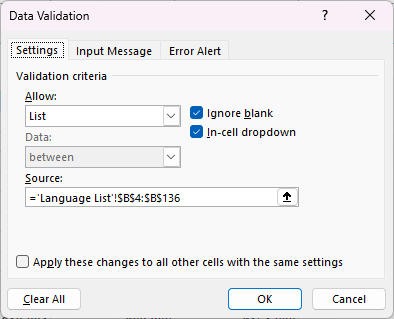
- Go to the Data tab on the ribbon and click Data Validation.
- In the Data Validation window, select List from the dropdown.
- In the Source field, select the range of cells that contain the languages you prepared earlier (the entire language column).
- Click OK, and your dropdown list is now ready!
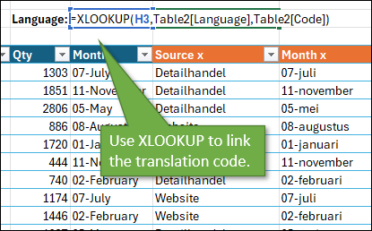
- Link to the Translation Code:
- Use XLOOKUP to match the selected language from the dropdown to its corresponding code (e.g., “en” for English, “fr” for French). This code will drive the translation in your report.
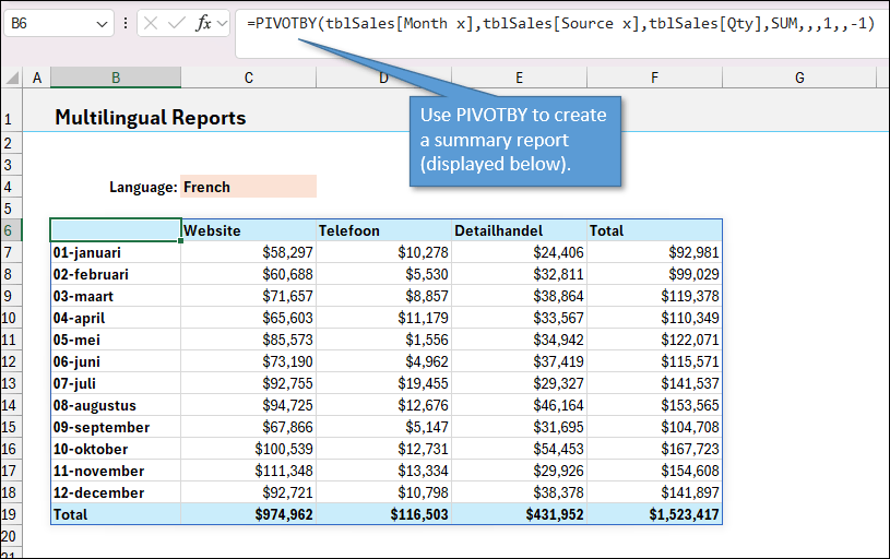
Using the PIVOTBY Function for Summary Reports
The new PIVOTBY function simplifies creating summary reports by automatically grouping your data. Here’s how to set it up:
- Select your Row Fields (translated Month column).
- Set your Column Fields (translated Source column).
- Select your Values (Qty column).
- Finish with a SUM to generate the summary.
This functionality allows you to present the same report in different languages without manually adjusting data.
For more about how to use PIVTOBY, check out this tutorial.
Note: If you want to create a chart from your data, be sure to translate the Chart Title using the TRANSLATE function as well. You can also wrap it in the PROPER function to ensure that all of the words translated are capitalized. See the video above for details on this technique.
Optimizing Performance
One challenge with translating large datasets is performance. To optimize your report:
- Create a Translation Table with unique values instead of translating each cell individually. Follow the steps in the video to create this table using Power Query.
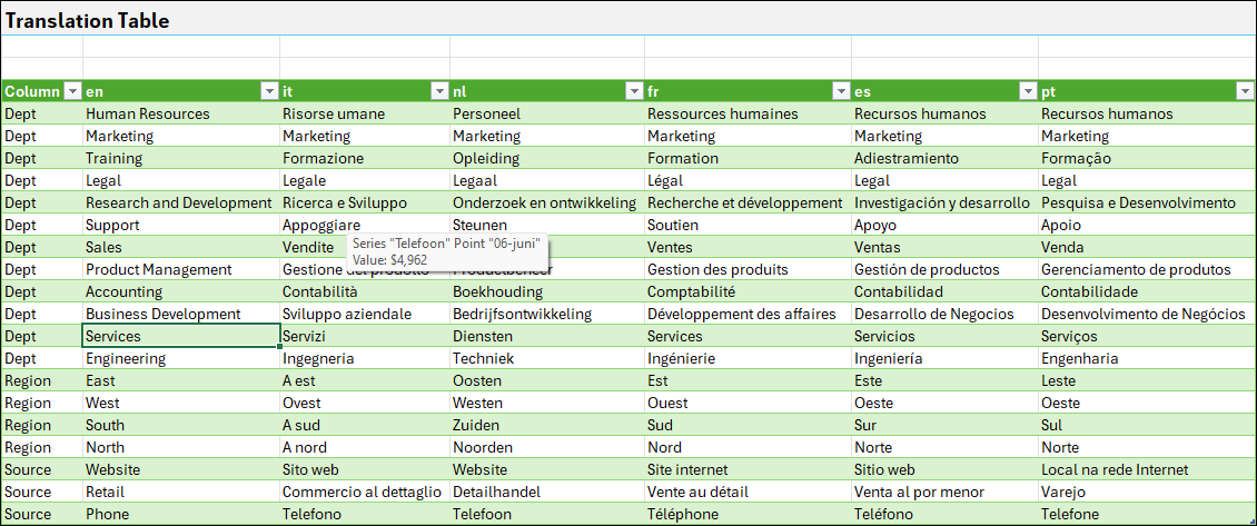
2. Use XLOOKUP twice to reference this table in your Customer Data—first to find the word in the original language, and then to pull the corresponding translation based on the selected language. This method drastically reduces redundant translations and improves efficiency, as it eliminates the need to translate each cell individually. (See the video for a breakdown of the XLOOKUP arguments.)
For more details on how to use Power Query, check out this post: Power Query Overview: An Introduction to Excel’s Most Powerful Data Tool
Offline Translation with XLOOKUP
The TRANSLATE function requires an internet connection, but you can make your reports offline-ready by preloading translations into a lookup table. Simply use XLOOKUP to pull from this static table instead of relying on the translation service.
This technique ensures that your reports function even when offline, making them more versatile.
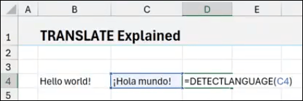
Bonus: DETECTLANGUAGE Function
If there is text in a language that you can't identify, you can use the DETECTLANGUAGE function to return the language code. Use your language list to match the code to the language so you can tell what language you are looking at.
Conclusion
With Excel's new translation features, creating interactive and dynamic reports in multiple languages is easy. Whether you’re managing data for international teams or optimizing reports for multilingual audiences, these new tools allow you to streamline your process and improve your workflow.
Do you see yourself using the translation functions? Leave a comment below and let us know what you think.


Great post of a very practical way to use =TRANSLATE / XLOOKUP.
Believe this is still in Insider / Beta channels. Same with PivotBy, GroupBy, PercentOf
Do you know when these will become available in General channel?
The download files linked (3) are for the Reconciliation video.
Couldn’t find the follow along file(s) for this video.