Bottom Line: Learn how to set up a “Show Details” checkbox using advanced Excel formulas and functions.
Skill Level: Advanced
In response to requests from our previous post on checkboxes, today we’ll dive into how to set up a “Show Details” checkbox in Excel. This is a fantastic opportunity to practice advanced formulas and work with helpful Excel functions like FILTER, INDEX MATCH, XMATCH, and EXPAND. So, let’s get into it!
Watch the Tutorial
Download the Excel File
You can follow along using the same Excel file that I used in the video.
What is the “Show Details” Checkbox?
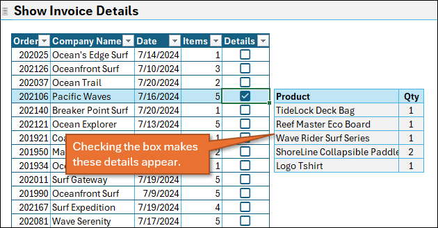
What do I mean when I talk about a Show Details Checkbox? Simply that when you click a checkbox, it reveals itemized details pertaining to the row that has the checkbox.
Examples you'll find in the Excel file inlcude:
- A checkbox that allows you to display detailed line items for an invoice when checked.
- A checkbox showing phone numbers for customers.
- A viewer-inspired checkbox showing expense details for projects.
Creating these checkboxes uses a combination of conditional formatting and a single formula to make everything work smoothly.
Setting Up the Show Details Checkbox
Here’s a quick overview of what you’ll need for the invoice example:
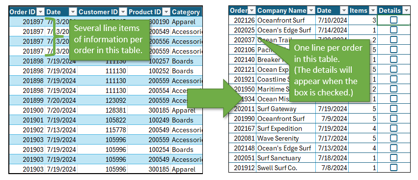
- Two Tables: One with all orders (unique order IDs) and one with the line items or details related to those orders.
- Checkboxes: You’ll need to be on a version of Excel that supports the new checkboxes feature. See this Microsoft article for details.
- Some Advanced Functions: You’ll be using a mix of Excel’s advanced functions to make this checkbox work effectively.
Step-by-Step Formula Walkthrough
- Start with the
FILTERFunction
Firstly, theFILTERfunction is key to returning all relevant details for the selected order. This formula looks at the selected order and pulls all related product names and quantities. You can modify it to return other columns as needed. - Integrate the Checkbox
To ensure that the checkbox drives this process, we modify the formula usingINDEXandXMATCH. This ensures that only the line items for the checked order are displayed.XMATCHfinds and returns the row number of the checked checkbox toINDEXfor theFILTERcriteria. - Align the Results with the Checkbox
Next, you’ll want the details to show up right beside the corresponding checkbox. This is where theVSTACKandEXPANDfunctions come into play, allowing the results to “spill” down the correct number of rows.EXPANDallows us to return a range of blank rows above the details table.
TheDROPfunction allows us to shift the range up to be in exact alignment with the checkbox row. - Improve formula efficiency.
SinceXMATCHis being calculated twice within the formula, we can useLETto streamline it.LETallows us to specify variables that hold the results of a calculation and use the variables multiple times throughout the larger formula. - Remove unsightly error message.
If no checkboxes are checked, the formula will return a #N/A error. To replace this with a blank cell, we can wrap everything in theIFERRORfunction. - Add Conditional Formatting
Finally, applying conditional formatting gives the table a clean, professional look. When the checkbox is checked, the corresponding details are highlighted, making it easy to focus on the selected data.
Be sure to watch the video (above) to see the formula built out step by step.
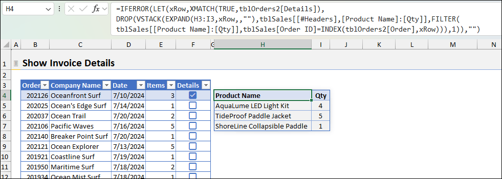
You can see how the final formula looks in the image below, as well as how those details look when you've checked a checkbox:
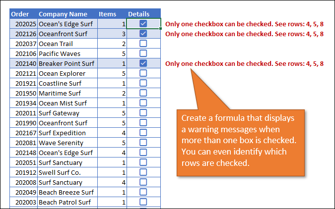
Checking Multiple Checkboxes
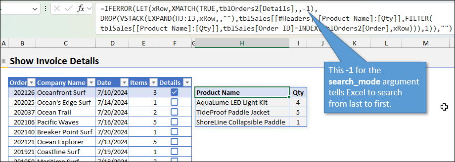
What happens when you check more than one checkbox? By default, the formula will return the results for the first checked box. However, you can modify this behavior to handle last-to-first matches.
XMATCH has a fourth argument called search_mode that changes the order of how the search is conducted. By going from last to first, only the lowest checked box in the list will display details.
Another alternative is to show an error message if more than one checkbox is checked.
Conclusion
The Show Details Checkbox provides a dynamic way to present detailed data in your Excel workbooks without clutter, making your spreadsheets much more interactive and user-friendly.
Are you planning to use this in your projects? Let us know in the comments!


Hi Jon, thank you so much for sharing it with us. This new functionality is incredible and although l haven’t watch the video yet (I am sure it is nothing short of fantastic) the explanation steps in text are fantastic indeed. I already decided that I will try to use it straight away in my new project tomorrow morning. I was wondering that would it be possible to incorporate “Show Details Checkbox” to the last column of a pivot table (as values in that column change when the pivot table refreshes). Thank you again Jon, have a nice week!
With a few lines of code, (and by saving the file as .xlsm) you can make the table only process 1 checkbox at a time:
Put this in the Sheet.Module
Private Sub Worksheet_Change(ByVal Target As Range)
Dim bln as boolean
Application.EnableEvents = False
If Not Intersect(Target, ActiveSheet.ListObjects(1).ListColumns(5).DataBodyRange) Is Nothing Then
bln = Target.Cells(1).Value
ActiveSheet.ListObjects(1).ListColumns(5).DataBodyRange.Value = False
If bln = True Then Target.Cells(1).Value = bln
End If
Application.EnableEvents = True
End Sub
Thanks for sharing it. Works great.
Hi Jon
Great Tut!! I will be utilizing this in my recipe collection to show ingredients. I have added formulas to the right (Col J etc) to include Index / Match forbringing in qataties based on the portion size I am catering for, as well as to check my food costings based on latest purchase pices.
WINNER WINNER, not just chicken a dinner bt steak too!!