Bottom Line: Learn how to create custom functions with the new LAMBDA feature of Excel. This post covers everything you need to know to get started, best practices, using LAMBDAS in other workbooks, and more.
Skill Level: Advanced
Watch the Tutorial
Download the Excel File
Follow along using the same file you see in the video. You can also copy the function we create in the video into your own workbook from this one, if you think it would be useful for your projects.
LAMBDA – An Exciting New Function
There's lots of excitement in the Excel world over a great new feature called LAMBDA. It's actually a function that allows you to write your own functions. (As of now, this is only available on the Insider's channels for Microsoft 365 users, but will roll out to other channels in the future.)
Creating functions that aren't already in the Excel function library can allow you to reuse and share custom functions that are unique to your industry, work type, or personalized projects. I want to show you an overview of how this new function works using an example inspired by Rob, a member of our Elevate Excel training group.
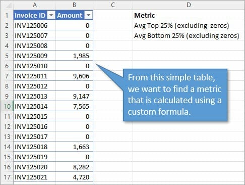
Rob's company often uses a performance metric calculated by taking the top 25% of entries from a data set (excluding zeros) and averaging them. This can be a fairly complex formula to write, and when transferring it to new reports, cell references and values need to be updated to make it work, which can potentially lead to mistakes and obviously takes some time.
It would be great if Rob and his fellow users could have a simplified function where only a couple of factors need to be identified—a function that can be used on any workbook by any user. That's where LAMBDA comes in.
Writing a LAMBDA Formula
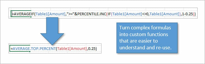
With LAMBDA, we can actually write a custom formula called, say, AVERAGE. TOP. PERCENT that averages a specified portion (such as the highest 25%) of a range and excludes zeros. Let's look at how that's done.
Note: We had to add spaces after each dot in the custom function name (AVERAGE. TOP. PERCENT) for email filter purposes. However, the actual function name in Excel cannot contain spaces.
Copy the Existing Calculation
The first step is to copy the existing formula for whatever you are trying to accomplish. In our example it is an AVERAGEIF function that excludes zeros before pulling out the top 25% of values and averaging them. It looks like this:

This formula is going to be pasted into our LAMBDA function as one of its arguments.
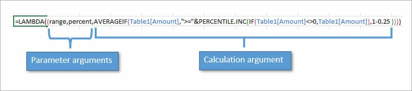
LAMBDA has two arguments: Parameter and Calculation. We want to paste this existing formula into the Calculation portion of the LAMBDA function.
Set Parameters
To define the Parameters argument, we must identify the inputs that we will feed into the calculation for the formula.
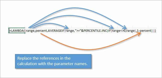
In our example, we want to replace Table1[Amount] with a variable name so that we can use it in other places. We will call that variable Range. We also want to replace the percentage with a variable so that we can change it whenever we write our new function. That variable we will call Percent.
So our LAMBDA formula, including the parameters and the calculation arguments, all together looks like this:
Next, we want to replace the parameters within the calculation with the new parameter names.
Pro Tip: Making the parameter names descriptive will help you to keep things straight as you put together your LAMBDA function. I do NOT recommend using parameters names like x, y, and z because you will have to take extra steps to figure out what the parameter names are used for when writing formulas.
Two Ways to Assign Values to the Parameters
At this point, Excel doesn't know what values to give to Range and Percent, so the LAMBDA formula returns a #CALC! error.
We have to tell Excel what we want the parameter values to be. There are two ways to go about this.
1. Create a Custom Function Through the Name Manager
Start by copying your entire LAMBDA function text. Then go to the Formulas tab and select Define Name.
That will bring up the New Name window where you can fill in the Name and Comment fields. It's a good idea to make note of the Range and Percent parameters in the comments.
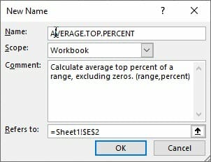
Then paste the LAMBDA function into the Refers to field.
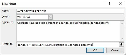
Hit OK. That's all you need to start using your new function. In any blank cell type the equals sign (=) and begin to type the word Average. You will see that the new function you created (AVERAGE. TOP. PERCENT) is in the list of available functions.
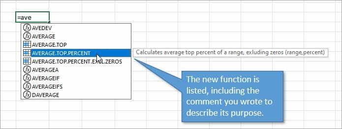
As of right now, when you start filling out the function by selecting the arguments, the screentip that usually shows the arguments for a function does not appear. That's why I had you write them into the comments, reminding you of what you need before you select the parameters.
So once you have tabbed into the AVERAGE. TOP. PERCENT function you can type the open parenthesis, select the range, type a comma, and then either select a cell that has your percentage in it or just type the percentage as a decimal (such as 0.25). When you close the parentheses, your completed formula should look like this:
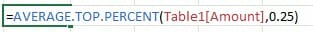
When you hit Enter it will return a value that averages the top 25 percent of your range, excluding zeros.
2. Add the Parameters in Parentheses After the Formula
The second way to tell Excel what values to use for the parameters is to write them after the formula in parentheses. See the highlighted portion below.
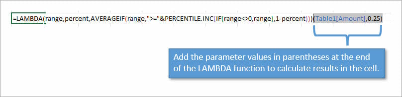
As long as they are written in the same order that they appear in in the formula, those values will feed into the formula correctly.
This second method might be better to use while creating and testing your function before going to the New Name window to name the function.
Altering your LAMBDA-Created Functions
To make edits to the functions you created using LAMBDA, go to the Name Manager button on the Formulas tab to bring up the Name Manager window. (Keyboard shortcut: Ctrl + F3.) There you will see a list of the functions you've created.
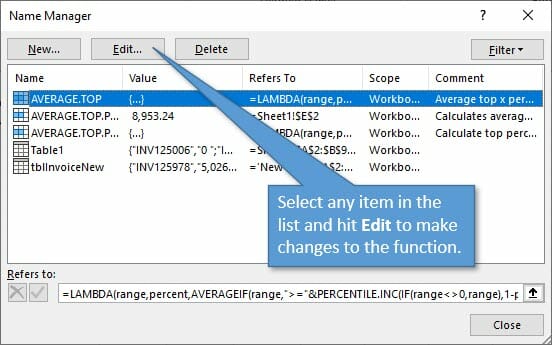
You can choose any of the items in the list to make modifications to its name, comment, or formula.
Reusing LAMBDAs
One of the great benefits of creating functions using LAMBDA is that they are reusable in other worksheets and workbooks.
The Same Workbook
To use the custom LAMBDA function in the same workbook, you just write the formula with your function name and add references or values for your arguments (range and percentage in this example). Since the named range is scoped to the workbook, the function will be available on any sheet in the workbook.
Other Workbooks
It's important to
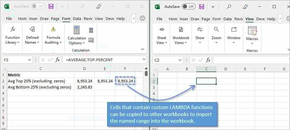
One important thing to note is that since the named range you created resides in the workbook that you created it in, you will NOT find it listed in your functions options in a other workbooks.
That's easily corrected by just copying a cell that contains the function from your original workbook and pasting it into the new workbook. That will import the named range into the new workbook. You will then see the function name in the formulas list when writing a formula.
If your function contains range references, then the formula that is pasted to the new workbook will contain links back to the original workbook. You can either delete the formula after pasting it or modify the references to ranges in the destination workbook.
If you have multiple LAMBDA functions in a workbook that you want to import into a new workbook, you can also copy the sheet tab to the new workbook. Just note that this will copy over ALL named ranges that are scoped to the workbook in the original workbook. If you use named ranges for other things, then you might not want this.
Conclusion
At this point, creating LAMBDA functions probably falls in the realm of advanced Excel users. But reading, understanding, and inputting formulas with most LAMBDA-created functions can easily be done by beginning and intermediate users.
As I mentioned previously, it will be much easier for the average user to read and understand the AVERAGE. TOP formula versus the complex AVERAGEIF formula that we started with. Even advanced users will spend less time trying to decipher complex formulas.
I believe this new feature has the ability to change how we use formulas in Excel, and I'm anxious to see how it evolves over time as it becomes more user-friendly.
I'd love to hear what you think about LAMDA and how you think you might be able to use it in your projects. Leave a comment below to let us know.
Related Posts
If you like this new LAMBDA feature, I think you'll like these other posts as well:


Very god!
Thanks for your documentation on LAMBDA. Have written a formula(works well) that uses LET Function to assign variables but cannot convert it to use LAMBDA
What I am wondering the most about LAMBDA is whether it is limited to the TWO parameters I see in all the examples, or if there is some other limit (say, up to 127 parameters, with the material after the last comma (semi-colon some places) being the formula, by definition (same model then as LET in that regard), or even 255 parameters, or no limit at all?
HOPING it is more than just two measly parameters. Don’t want to have to pull out the 1890’s kid’s hoops and start them rolling to the center circle of the Big Top and commence jumping through them before I even have the honor of someday getting the function rolled out to me…
Be nice too, if someone wrote a macro that would take the name of your LAMBDA’s Named Range (there WILL be one, or it’s just a (possibly, see above) crippled LET), the comment, and the “Refers to” and places them in a standard worksheet (“standard” because the macro would pick a name for it (and .xlsx) and no one would ever change it so as to make the macro universal, create it if it did not exist (perhaps wherever your PERSONAL workbook WOULD be stored, or is), and record these things in a row in the standard for all time and places workbook. Perhaps other details like the file it came from.
In any case, the other function of the macro would be for you to select a cell in the standard workbook and activate it, whereupon it would take those pieces of information, pause for your response to “Please select the currently open workbook to add this too” which you would do via mousing to that window, and create the Named Range with the LAMBDA in the indicated open workbook with workbook scope.
It could be dressed up with niceties like changing literal references absolute (which you could edit later) and when creating the row, creating sub-rows for any Named Ranges it found as dependencies (a macro ought to be able to see Named Ranges in the LAMBDA). Not necessarily going more than that one level deep for that!! Another might be figuring the “box” for all ranges referenced (so, C1:K3, D7:AA12, H26 might give a “box” of C1:AA26 that would let the macro change the references so the upper left corner of the “box” would not be C1 but rather A1… it’d give maximum ease in moving it around in the new spreadsheet, though clearly it’s like a 2nd or 3rd level nicety and hardly necessary, not 1st level like the literal references to absolute literal references thing. For 4th level, it might anchor the box to any already absolute references found, and report the upper left corner cell for that.
Anyway, if it just did the not-dressed-up-with-niceties part, it could be the first almost universal macro anyone ever wrote. And maybe (yeah, “maybe”) shame MS into adding the functionality in real code, and providing some of the bells and whistles.
“Shamed” because the fact they don’t seem on track to offer anything like that suggests they figured it way too hard, and a kinda basic, though involved macro performing the work for them, they work they found too hard with real, integrated code…
Or as an Add-In, so even the standard, universal, workbook with it and your LAMBDA LIBRARY would not need to be a macro spreadsheet…
But DO tell me that it will take more than two parameters without hoops…
(A “hoop” might be like, it takes the two parameters, but like some formulas with limited parameter quantity, each parameter can actually refer to somewhere that contains a LONG list of more parameters, effectively making the total one can give it infinite-ish. (Only some are like that, and not really useful for parameters that are different “kinds,” rather more for just giving SUMIF, perhaps, a thousand parameters, all the same KIND, rather than whatever its “natural” limit is.) One kind of hoop. Another would be what to do if, as one expects, it won’t take ranges greater than one dimension. That one’s a lot more involved, though, than the first. Other hoops might be somewhat in between.)
Funny though, that the recommended form of usage is essentially giving parameters to Named Ranges which I’ve been doing for nearly 25 years. Assuredly, taking the parameters natively and accepting all types Excel accepts will be hideously nicer than incredible effort to take most or limiting the input you accept (not actually a problem when written for yourself only, but when for a boss or a whiner…). And using it directly instead of wrapped in IFERROR, so nice, and acceptable to others. But mostly, the composition time will be seconds rather than an hour spent working out each one’s details, possibly choosing at some point to limit parameter types, going back and working the details through again…
And now that MS is actively taking steps to pull fans away from ever using the Excel 4 Macros anymore (at least two major steps recently), the writing was on the wall anyway. Makes one think they actually knew about it too and now that LAMBDA is close for us hoi polloi, they will rapidly cut it once and for all.
If they do, they’d BETTER create a cell-side EVALUATE first. Unless LAMBDA will also accept a FORMULATEXT-style string as input — i.e.: let you build your formula AS A STRING, then treat the result as a literally written formula — in which case, much of the need for EVALUATE would finally go away. But given they still won’t write a formal function to take “pieces parts” (cells and ranges, dis-contiguous ones, specified to it) and make a true, single, array of them directly (basic purpose of the function!)… I WORRY…
Found MS documentation that answers my “How many parameters are available?” question: 253.
So cool, that’s very, very nice.