Only Display Used Fields on Pivot Table Show Details Sheet

Bottom line: Learn how to create a Show Details Drill Down Sheet from a pivot table that only contains the fields (columns) used in the pivot table.

Skill level: Intermediate

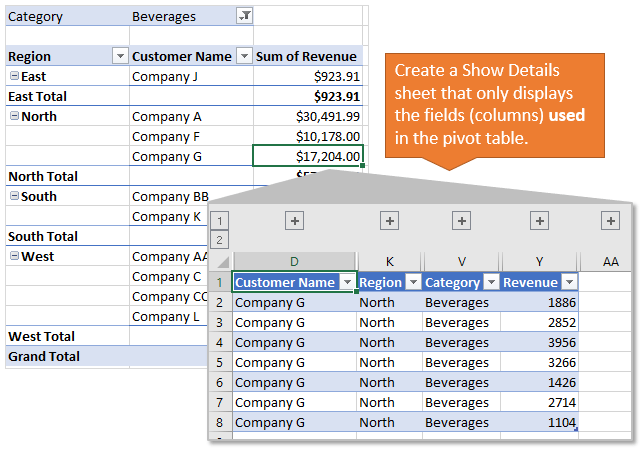
The Show Details Sheet Usually Shows All Fields

When we double-click a cell in the values area of a pivot table (or right-click > Show Details), a new sheet is added to the workbook.  The new sheet contains all of the source data rows for cell we double-clicked.

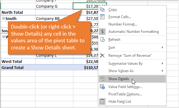
This can be useful when you are tying out numbers and want to see all the rows that make up a specific number.

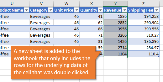
The show details sheet also contains ALL of the columns from the source data range.

Aris, a member of the Excel Campus community, asked a great question and wants to know if we can create a details sheet that ONLY includes the fields used in the pivot table?

This isn't directly possible in Excel, but we can use a macro to solve this problem.  Let's see how we can use VBA to save the day (and save a ton of time)! 🙂

The Show Details of Used Fields Macro

The following macro will group and hide or delete columns in the Show Details sheet that are NOT used in the pivot table.  This means we will be left with a show details sheet that only contains the fields (columns) that are used in pivot table.  This gives us a much skinnier table that can be easier to read.

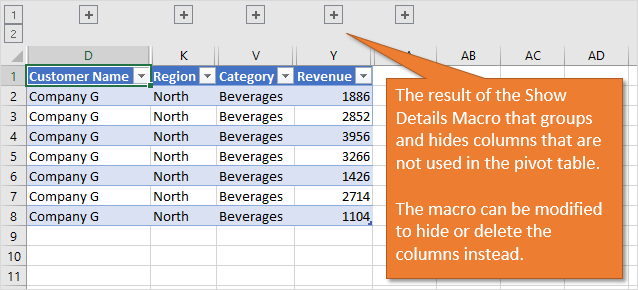
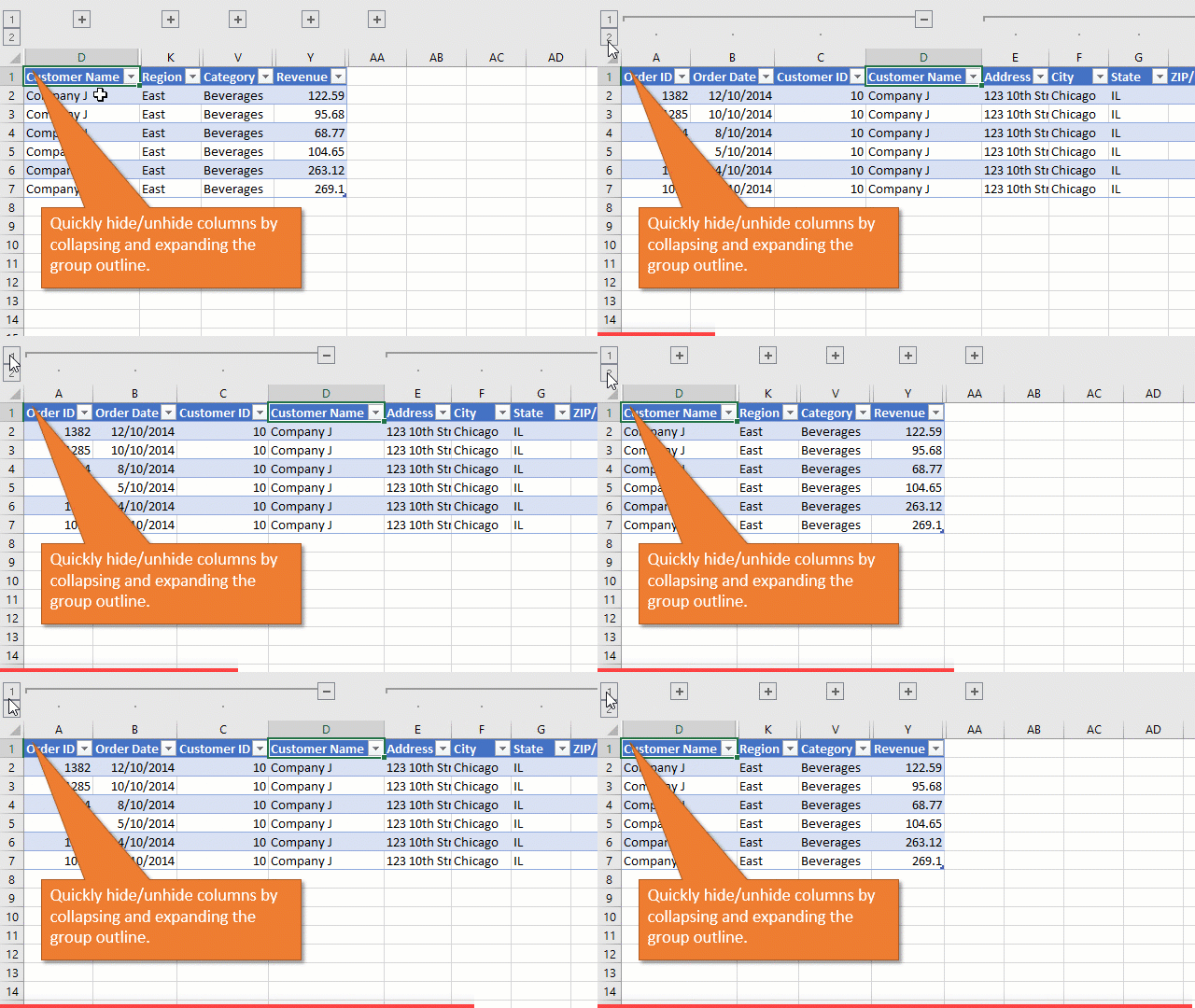
The advantage of grouping and hiding the columns is that they can easily be made visible by pressing the 2 in the top left corner to expand the groups.

How Does The Macro Work?

Here's what happens when you run the macro:

1. The macro creates the ShowDetails sheet for the active cell in the pivot table.
2. It then loops through each column in the Table (List Object) of the new sheet.
3. It checks to see if the column (field) is used in any of the areas in the pivot table.
4. If the column is NOT used then it groups the column (columns can also be hidden or deleted).
5. Steps 3 & 4 are repeated for each column.
6. The column outline is collapsed so only the used columns remain visible.
7. The columns widths of the Table are auto fit, which saves another step with the show details sheets.

Download the Excel File

Download the file that contains the macro.

Here is the macro that you can copy & paste to your Personal Macro Workbook or any VBA Project.

Sub Show_Details_Used_Fields_Only()
'Creates a Details Sheet for a Pivot Table
'based on the activecell and Deletes or Hides
'columns that are not used in the pivot table.
'The macro can be added to your Personal Macro
'Workbook and be run on any open file.
'Source:  https://www.excelcampus.com/vba/pivot-table-show-details-used-fields-only

Dim pt As PivotTable
Dim pf As PivotField
Dim pfData As PivotField
Dim lo As ListObject
Dim loCol As ListColumn
Dim bVisible As Boolean

    
  'Check the activecell is in a pivot table
  On Error Resume Next
  Set pt = ActiveCell.PivotTable
  On Error GoTo 0
  
  If pt Is Nothing Then
    MsgBox "Please select a cell inside a pivot table"
    Exit Sub
  End If
  
  'Check the activecell is in the values area of a pivot table
  If Not Intersect(ActiveCell, pt.DataBodyRange) Is Nothing Then
  
    'Create the show details sheet
    ActiveCell.ShowDetail = True
    
    'Set ListObject (Table) on show details sheet
    Set lo = ActiveSheet.ListObjects(1)
    
    'Delete unused columns from the details sheet
    For Each loCol In lo.ListColumns
      
      bVisible = False
      
      'Check the field is not used in the Filters, Rows, or
      'Columns areas
      For Each pf In pt.PivotFields
        If pf.Name <> "Values" Then
          If pf.SourceName = loCol.Name Then
            If pf.Orientation = xlHidden Then
              'Check the field isn't used in the Values area
              'DataFields in the values area have a Hidden Orientation
              For Each pfData In pt.DataFields
                If pfData.SourceName = loCol.Name Then
                  bVisible = True
                End If
              Next pfData
            Else
              'Field is used in rows, cols, or filters areas
              bVisible = True
            End If
            
           'Group and collapse the columns in the details sheet
            If bVisible = False Then
              'Uncomment any of the lines below to delete or hide
              'the columns instead of grouping
              loCol.Range.EntireColumn.Group
              'loCol.Delete
              'loCol.Range.EntireColumn.Hidden = True
            End If
          End If
        End If
      Next pf
      
    Next loCol
    
    'Collapse groups
    ActiveSheet.Outline.ShowLevels ColumnLevels:=1
    
    'Autofit columns
    lo.Range.SpecialCells(xlCellTypeVisible).EntireColumn.AutoFit
    
  Else
    MsgBox "Please select a cell in the values area of the pivot table."
    Exit Sub
    
  End If

End Sub

How to Run the Macro

Download the file that contains the macro.

The macro can be added to your Personal Macro Workbook and run on any Excel file you have open. You can add a button to the ribbon that will run the macro any time. Checkout my free video series on the Personal Macro Workbook to learn how to get started and create the ribbon buttons.

We could also add a button to the pivot table's right-click menu to run the macro. I shared similar code in my article on Automatic Default Number Formatting for Pivot Tables, but please leave a comment below if you are interested in the code to add a button to the right-click menu.

Another option is to add the code to an App Event for the BeforeDoubleClick event. Then the macro could automatically run when a cell in double-clicked in the pivot table.

There are a lot of ways to implement this macro, depending on how often you want to use it.  Please leave a comment below with any questions or suggestions on how to improve it.  Thank you! 🙂

How to Learn Excel Macros

If you are interested in learning more about macros, I’m currently running my free webinar called “The 7 Steps to Getting Started with Macros & VBA”.

During the webinar I explain why you might want to learn VBA, and a lot of the basic coding concepts that will help you get started. I jump into Excel and the VB Editor and walk through how to write and run our first macro. Even if you have been using VBA for awhile, I’m sure you will learn some new tips.

Click here to register for the webinar, it's FREE!