2 Ways to Reverse Number Signs Positive Negative in Excel

Bottom line: Learn 2 ways to reverse the sign of a number from positive to negative or negative to positive in Excel.

Skill level: Beginner

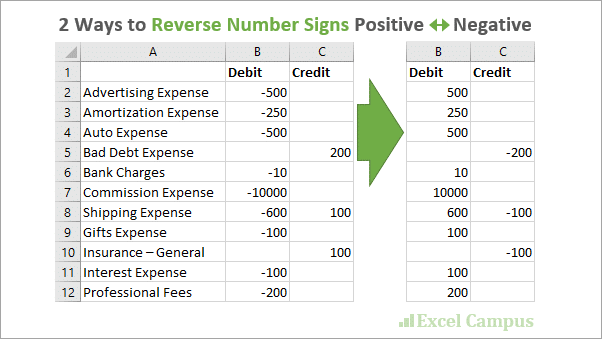
My friend Robbie asked a great question on how to reverse the number signs in Excel.   He had a journal entry sheet with a list of debits and credits that was exported from bank system.  The numeric values needed to be flipped positive <-> negative for the general ledger accounting system he is using.

Like everything in Excel, there are a few ways to solve this problem.  In this article and video we look at how to reverse the signs with a formula and with the Paste Special menu in Excel.

Video: 2 Ways to Reverse Number Signs Positive Negative

Method #1 – Multiply by Negative 1 with a Formula

The first method is pretty simple.  We can write a formula to multiply the cell's value by negative 1 (-1).

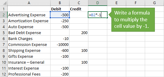
This works on cells that contain either positive or negative numbers.  The result of the formula is:

• Positive numbers will be converted to negative numbers.
• Or negative numbers will be converted to positive numbers.

We can then copy/paste the formula to get the results for all the cells in columns B & C.

Method #2 – Paste Special Multiply Operation

The first solution with the formula works great, but is forces us to create new columns of data that contain formulas.  We might want to just change the existing values in columns B & C instead.

This can be done with copy and paste.  We will copy a cell that contains a -1, then use the Multiply operation on the Paste Special menu.  This will perform the multiplication on the selected cells that we paste to.

Here is a quick screen cast animation that shows how to perform the Paste Special operation.

I explain this in more detail in the video above, but here are the steps to reverse the number sign using Paste Special:

1. Type -1 in a blank cell on the worksheet.
2. Select the cells that contains the -1 and copy it.
3. Select the cell(s) that contain the numbers you want to reverse.
4. Open the Paste Special menu: Right-click > Paste Special… (Alt,E,S)
5. Click the “Multiply” radio button in the Operation section of the Paste Special menu.
6. Press OK.

All of the values in the selected cells will be multiplied by -1.  The result is that the signs will be reversed for each cell value.

Only Reverse the Sign in the Non-blank Cells

In our original example column B & C contain some blank cells.  If we select all the cells in the range including the blank cells, then do the paste special, the blank cells will converted to 0 (zeros).

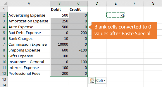
Now, we might want to keep those blank cells blank.  We can do this by using the Go To Special menu to first select non-blank cells (constants/formulas) before performing the paste.

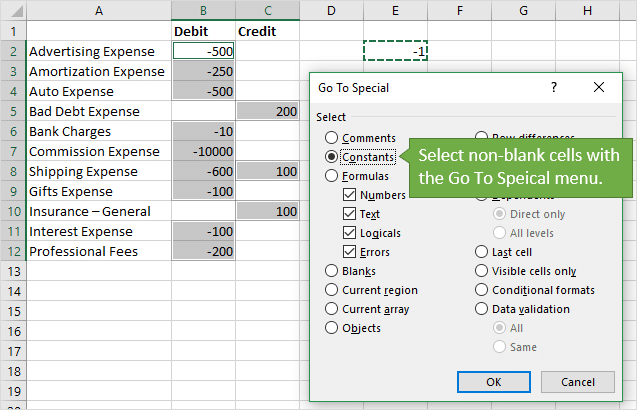
I explain this in more detail in the video above, but here are the steps:

1. Copy the cell that contains the -1.
2. Select the range to paste to, including the blank cells.
3. Open the Go To Special Menu (Home tab > Find & Select > Go To Special…)
4. Click the Constants radio button to select cells that contain values (non-blank).
5. Press OK.
6. The cells that contain values (non-blanks) will be selected.
7. Perform the Paste Special Multiply operation (Right-click > Paste Special > Multiply > OK

This time only the selected cells will be multiplied by negative 1 to reverse the sign.

Only Reverse the Sign on the Visible Cells

We can use the Paste Special Multiply operation on a filtered range as well.  We will first want to select the visible cells only on the filtered range.  This can be done on the Go To Special menu or with the keyboard shortcut Alt+;

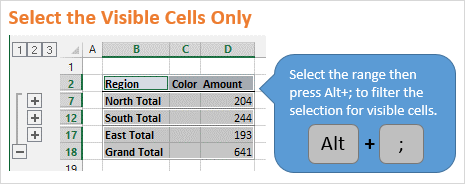
Checkout my article and video on how to copy and paste the visible cells only for more details on this technique.

Reverse the Sign in Cells that Contain Formulas

The Paste Special Multiply operation also works on cells that contain formulas.  The cells in the example below contain a VLOOKUP formula.  We might want to reverse the signs of the results, but also keep the formula.

When we perform the paste special on a cell that contains a formula, the formula is modified to add a *-1 to the end of it.  That means we do NOT lose the formulas.

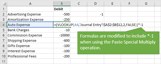
We can also use the Go To Special menu here to first select cells that contain Formulas (non-blanks) before performing the Paste Special.

Keepin Your Sheets Positive

Well, there are two ways to reverse the number signs in Excel.  This is a common task when exporting data from financial systems, and needing to flip the signs for journal entries (debit and credits).

What techniques do you use to reverse number signs?  Please leave a comment below with any questions or suggestions.  Thank you! 🙂