2 Ways to Filter for List of Items in Excel + Video Tutorial

Bottom line: Learn 2 ways to filter for a list of multiple items in Excel in this article and video tutorial.

Skill level: Beginner

Video Tutorial

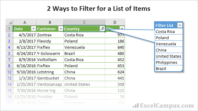
The following video is from The Filters 101 Course.  In this video I explain two ways to apply a filter for a list of multiple items.  These techniques use the Filter Drop-down menus in Excel.

Sample Video from The Filters 101 Course

The video above is from The Filters 101 Course.  Filters 101 is an online video course with over 40 video lessons like the one above.

Click here to learn more about The Filters 101 Course

Filtering for Multiple Items

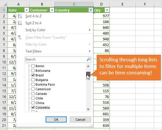
A few questions come in this week from Jennifer and Justin on how to apply a filter for a list of multiple items.  This can be a time-consuming task if you try to check all the boxes for different items in the filter drop-down menus.  Especially if the filter list contains a lot of items.

We find ourselves scrolling up and down the list to check each checkbox for all items in our list.  There are a few ways to speed up this process.  Let's take a look at two methods that can save us time.

Method #1 – Add current selection to filter

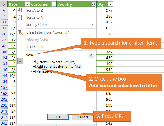
The first method for filtering for a list of items uses an option in the filter drop-down list box called “Add current selection to filter”.  As the name suggests, this feature allows us to use the Search box to search for an item, then add the selected items to the current filter criteria.

This technique works best when you have 3-5 items to filter for.  Here are the steps to use the Add current selection to filter method:

1. Use the Search box in the filter drop-down menu to search for the first item.
2. Click OK to apply the filter.
3. Open the filter drop-down menu again.
4. Use the Search box (keyboard shortcut: e) to search for the second item in your filter list.
5. Click the “Add current selection to filter” checkbox.
6. Click OK.  The existing filter criteria will be kept, and the new item will be added to the filter criteria.
7. Repeat steps 3 to 6 for each additional item in your filter list.

This process can be time-consuming if you have more than a few items in your filter criteria.  See the video above for further explanation on this technique.

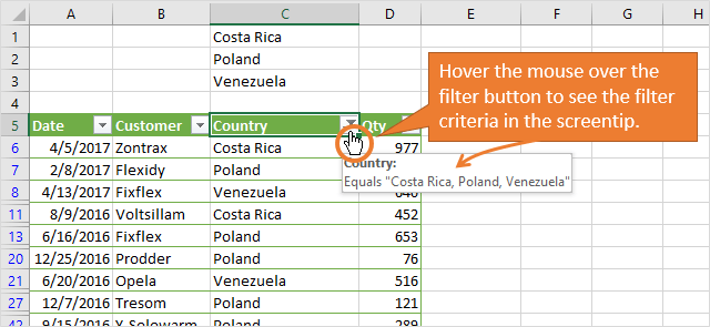
It's also hard to see what items have been filtered for by scrolling through the checkbox list.  One tip for this is to hover your mouse over the filter drop-down button.  A screentip will appear and display the filter criteria.

My Filter Mate Add-in will also help with viewing the filter criteria for the filter menus.  Check out my post on 7 Keyboard Shortcuts for the Filter Drop-down Menus for more time-saving tips on the filter menus.

Method #2 – Add a Column with a COUNTIF Formula

The second method is a formula based approach that works great for longer lists of filter items.

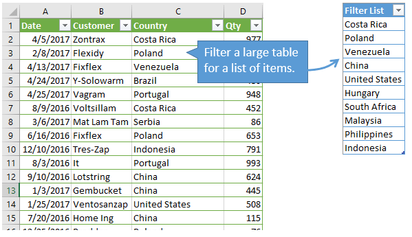
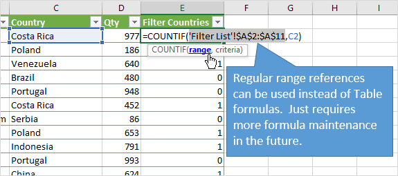
In this example, we want to apply a filter to the data table for a list of countries.  This means we only want to see the rows that contain ANY of the countries in the filter list.  We can add a column to the data table with a COUNTIF formula.

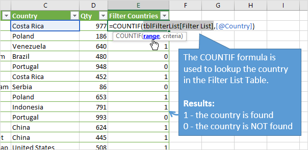
We use the COUNTIF formula to determine if the country name in the same row in column C exists in the filter list.  The filter list is the list of items that we want to filter for.  This list can be on the same sheet or a different sheet.

The formula will return:

• 1 if the country exists in the filter list
• 0 if the country does not exist.

We now have a column of 1's and 0's.

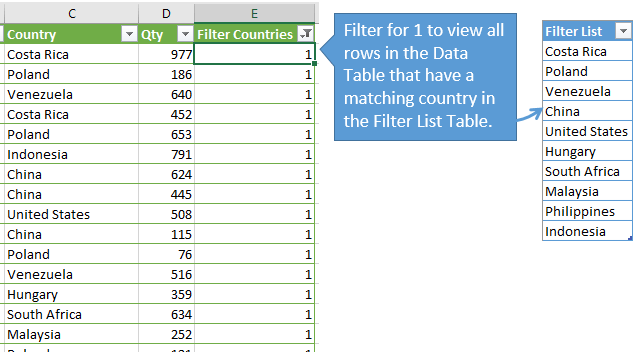
Finally, we can apply a filter to the column to filter for 1.  This filter will display all the rows where the country in column C matches a country in the filter list.

See my article on using COUNTIF instead of VLOOKUP for more details on the COUNTIF function.

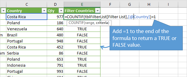
We can also add a “=1” to the end of the formula to return a TRUE or FALSE, instead of 1 or 0.

The TRUE or FALSE values will make more sense if you are using the field in a pivot table or slicer, and want to quickly apply a filter for the country list.  The TRUE/FALSE is just easier to read and understand versus the 1 or 0.  However, the outcome will be the same.  See my article on the IF function for more about this TRUE/FALSE boolean logic.

I use Excel Tables for this example.  You do NOT have to use Excel Tables for this to work.

The advantage of using Tables is that we can add new items to the filter list, and we don't have to modify the formula.  Since the formula references the entire column of the Table, there is not maintenance here.  We just need to Re-apply the filters (keyboard shortcut: Ctrl+Alt+L) after adding new items to the filter list.  This saves time and prevents errors.  Win-win! 🙂

Check out my video on A Beginner's Guide to Excel Tables to learn more about this awesome feature of Excel.

What about Partial Matches that Contain the Filter Criteria?

Arun had a great question in the comments below about filtering for partial matches that contain the filter criteria.  We are limited to 2 criteria with the Custom AutoFilter in Excel.

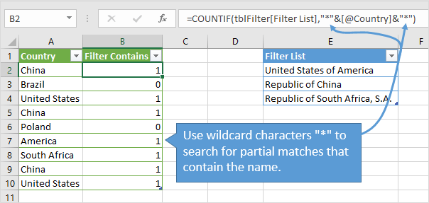
However, we can use this same COUNTIFS technique with wildcard characters to filter for partial matches that contain the criteria. Here is an example of how to modify the formula.

=COUNTIF(tblFilterList[Filter List],"*"&[@Country]&"*")

The asterisk character (*) is a wildcard character that represents any value.  To use the wildcard character in the COUNTIF function, we wrap it in quotation marks and use the ampersand symbol to join it to the criteria value.

The argument evaluates to *[@Country]*. This means that COUNTIF will look for the country name within the cell, and return a 1 if the name is found within a cell in the range.

The asterisk represents any number of characters before or after the country name. This is the same as a ‘Contains' type criteria. We can just put the asterisk at the beginning or end if we want to find matching cells that start or end with the lookup value.

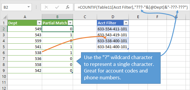
We can also use the “?” wildcard character to represent a single character.  Here is an example.

This works great for account codes and phone numbers.

What Techniques Do You Use to Filter Multiple Items?

These are two simple techniques to filter multiple items.  With everything in Excel, there are many ways to go about this.  Do you use a different technique?  If so, please let us know by leaving a comment below.  You can also leave a comment with any questions.

I also have a free 3-part video series on Excel Filters.  In video #3 of the series, we look at applying filters to multiple columns.

Check Out The Filters 101 Course

The video above is a sample lesson from The Filters 101 Course.  This course contains over 40 video lessons just like this one.  This is step-by-step training that will help you get the most out of the sort & filter features in Excel, to prepare & analyze your data faster.

Click here to learn more about The Filters 101 Course