Bottom line: Learn how to filter for a list of items using a reverse partial match lookup.
Skill level: Intermediate
Video Tutorial
Download the Example File
Download the example Excel file to follow along.
Reverse Partial Match Lookup
A few great questions came in from last week's post on 2 ways to filter for a list of multiple items.
Arun and Edil wanted to know how to filter a column for a partial match to any item in the filter list. We want to see if the cell in the data list contains ANY of the words in the filter list.
We can call this a reverse partial match lookup.
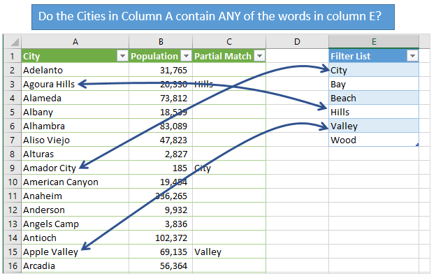
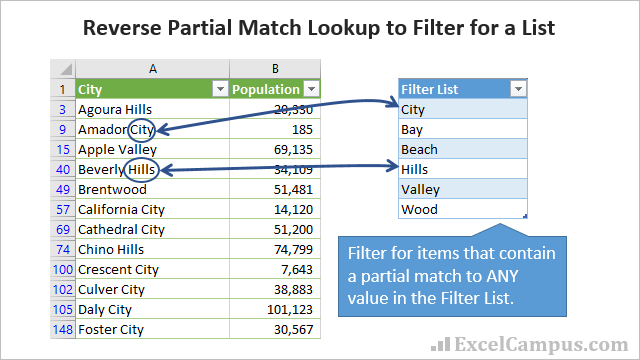
In this example we have a list of all the cities in California. We want to search the list of city names to see if each name contains ANY of the words in the filter list (column E). We then want to filter the city list for all partial matches to the filter list.
The LOOKUP and SEARCH Formula Explained
Like everything in Excel, there are a few ways to go about this. In this example we are going to use a formula with the LOOKUP and SEARCH functions.
Here is the formula. It's a bit of a monster. 🙂
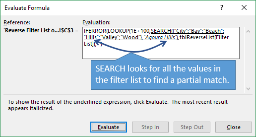
=IFERROR(LOOKUP(1E+100,SEARCH(tblReverseList[Filter List],[@City]),tblReverseList[Filter List]),"")
The formula uses the SEARCH function to look for each item in the Filter List within the cell that is referenced in the “within_text” argument. If the SEARCH function finds a match, it returns the character number that the search word (find_text) starts at.
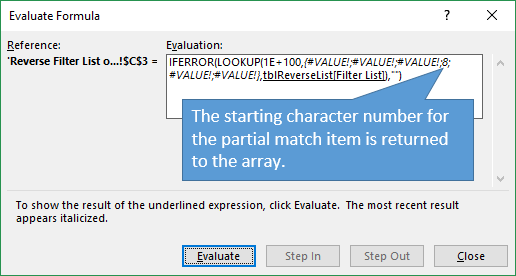
This returns an array (list) of values that looks like the following.
{#VALUE!;#VALUE!;#VALUE!;8;#VALUE!;#VALUE!;}
A number is returned in the list where a match is found. In the list above, the 4th item contains a match that starts at the 8th character in the word that is being searched.
The LOOKUP function is then used to find any numbers in the resulting array list from the SEARCH function. The lookup value is “1E+100”. This is scientific notation for a really large number. Since the number that is found will be smaller than that number, the LOOKUP function returns the last number in the list (array).
Since we specified the optional “result_vector” argument for LOOKUP as the filter list, LOOKUP returns the contents of the cell for the 4th item in the list.
The formula is then wrapped in the IFERROR function. If no matches are found, the LOOKUP function will return a #N/A error. The IFERROR function handles the error and allows us to return a blank or other value.

The SEARCH function is NOT case sensitive. This means it doesn't consider upper or lower case letters and will return a match even if the case doesn't match. We can use the FIND function, instead of SEARCH, to do a case sensitive search.
Checkout the video above for further explanation on this formula.
Filter The List for All Partial Matches
We can now apply a filter to column that contains the formula. Since the IFERROR function returns a blank “” if no partial match is found, we can filter out blanks to see all rows that contain a partial match.

We can also just return a TRUE or FALSE as the result of the formula to make filtering easier. To do this we just add the following to the end of the formula.
<>""
That means Does Not Equal Blank. So the full formula looks like the following.
=IFERROR(LOOKUP(1E+100,SEARCH(tblReverseList[Filter List],[@City]),tblReverseList[Filter List]),"")<>""
Now we can filter the column for TRUE to see all the cities that contain ANY of the words from filter list.
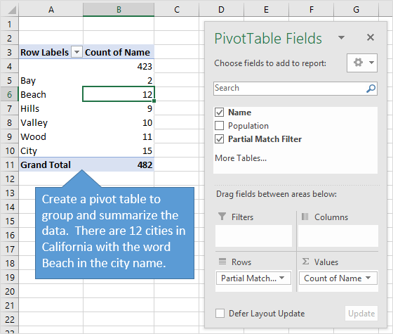
Group Items for Summary Reports and Pivot Tables
The column with the LOOKUP and SEARCH formula can also be used to group items in a pivot table. By adding the Partial Match field to the Rows area of the pivot table, we can quickly see a report of the total number of cities in California that contain one of the words in the filter list.
Check Out The Filters 101 Course
The Filters 101 Online Course contains over 40 video lessons just like this one. This is step-by-step training that will help you get the most out of the sort & filter features in Excel, to prepare & analyze your data faster.

Click here to learn more about The Filters 101 Course
How will you use this technique? Please leave a comment below with any suggestions or questions. Thank you! 🙂


Hi Jon,
Perfect and thanks a ton! Sincerely appreciate you taking time to add this new blog in response to my query in the previous edition.
This is exactly what I was looking for and is working with me. There is only one challenge which I am facing. The formula is throwing false results in case there are empty spaces in filter list (ie empty cell between E2 to E7). Any solution for this also..
Arun
Hi Arun,
Thanks! I’m happy to hear it helped.
You will probably want to remove any blank (empty) cells from the Filter List. If you are. Otherwise the formula will return a zero (0). You could handle the zero by adding
to the end of the formula. That will give you a column of TRUE/FALSE values.
But, it might make more sense to just delete the blank cells from the filter list if possible.
I hope that helps. 🙂
Thanks Jon, I will go by your suggestion by filling dummy values to avoid any blank cells in the filter list.
Hi Jon,
Simply awesome, your answer and explanation to my query.
I tried it out and “VOILÁ”, there are all the records I needed.
Thank you very much.
Awesome! I’m happy to hear it helped Edil. Thank you for letting me know. 🙂
Hello Jon,
Thanks for your great Excel help. I have been working with the example you gave in the video today, but I cannot make the Search function use multiple criteria in the find_text location (the Filter List.) Excel 2010 is the version I’m on; does this require the 2013 or 2016 release?
Sincerely,
Douglas Phelps
Hi Douglas,
The formula should work in Excel 2010.
Hi Jon, Why is it that the SEARCH function on its own will only find the value that directly corresponds to the value on the same row (even if that whole table is referenced), yet when used in conjuntion with LOOKUP, it searches through the entire list to get a match. I don’t see where the LOOKUP function changes how the SEARCH function works as it is just a parameter of the LOOKUP function. Example – your search list, in order is City, Bay, Beach, Hills, Valley, Wood and the City names are Adelanto, Agoura Hills, Alameda, Albany, Alhambra, Aliso Viejo. You will never get any results from those five Cities because the filter list item is not on the same row. If you add the word City of Adelanto, you will get a result.
Thanks Bernice
Hi Bernice,
Great question! The LOOKUP function converts the SEARCH function results to an array formula. Typically we would have to press Ctrl+Shift+Enter with the SEARCH function to perform this type of search on multiple cells. However, the LOOKUP function creates the array for us in the lookup_vector argument.
I hope that helps. 🙂
Thanks! That solved my question same as Bernice’s.
Hi Jon,
Kindly tell how to hide and secure our formula in excel which can not visible or edit without permission??
Hi Jon,
I have another way of doing it. I mean parse the list with space delimiter and you get all the city, hills values into separate columns without any lookup. And just filter what you need. I think this also does the same job without formula.
Any comments please.
Best regards
Eswari
Hi Eswari,
You are still going to need an additional column with a formula to filter for all rows that contain a match. It will also be difficult to use that method in a pivot table filter, as I explain in the video.
Thanks for the suggestion though! 🙂
That’s awesome and fascinating Mr. Jon
Thanks a lot
Thanks Yasser! 🙂
Wish me good luck to make this work on Google Sheet ^^
Hi,
It’s really nice! whereas while trying i found one more way out to resolve the query and i.e =IF(OR(RIGHT(F2,3)=$J$2,RIGHT(F2,4)=$J$3)=TRUE,F2,””)
F column has complete list of cities and J2 & J3 are the cells with the suffix of city names(i have considered only two suffix in place of multiple like you)
Your suggestion on this shall be highly appreciated!
Thank You
Hi Jon,
Great formula that I’m already using.
One question, if a city has more than 1 name from the filter list, for example “Bay City” then the formula returns the first item only, “Bay”. Is there a way to return and count both?
Tom
Hi Tom,
Great question. My friend Kevin wrote a follow-up post that explains one possible solution to count all occurrences.
That’s awesome Mr.Jon. Thank you.
Hi Jon,
How can I create a macro that will search for a partial match then copy the results to a new worksheet?
Thank you,
Florence
Great question Florence! I’ll add this to my list for future posts. Thanks!
Hi Jon,
I created a post to explore a couple of additional questions based on your partial match.
http://www.myspreadsheetlab.com/reverse-partial-match-lookup-to-filter-for-a-list/
Cheers,
Kevin
Hi Kevin,
Great article! Thanks for following up and sharing your alternate solutions. Awesome! 🙂
Jon
Hi Jon,
Nice formula!
With slight modification, we can do it in a non-formula approach – Advanced Filter.
Thanks for your inspiration for me to write a blogpost about Advanced Filter. Will share with you later here.
Happy Friday. 🙂
Hi Jon,
As promised this is my blogpost for sharing:
Filter a list of items from a long long list | wmfexcel
https://wmfexcel.com/2017/08/02/filter-a-lists-of-items-from-a-long-long-list/
Hope you and your readers like it.
Cheers,
Such brilliance, worked like a charm, Thank you…
Hi! Thanks for your article! It helped a loooot!
Just one question…. why does it not work when I “break” the formula in two steps? I tried in one cell to calc the Search and in the other, use the lookup with the value of the previous cell…
Thanks in advance! 🙂
Hello, great solution! Thanks for that. But what if we would like to get all the occurrences found separated by a delimiter? Or being able to choose the nth occurrence found?