Enhance Your Checkboxes with Conditional Formatting in Excel

Bottom Line: Learn how to create checkboxes where the text formatting changes when the checkbox is checked or unchecked. This makes it easier to see which items have been completed or which item is next to complete.

Skill Level: Advanced

View the Tutorial

Download the Excel File

Here's the Excel workbook that I use in the video. Download it and follow along!

Enhancing Your Checklist

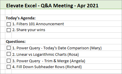
Today let's look at how to use conditional formatting to make your checklists better. For example, we can make the font gray for items we've checked off our list:

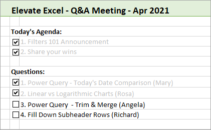
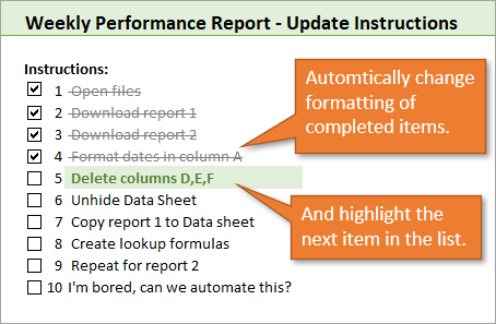
We can draw a line through checked items as well. Or we can even bring attention to the next item on the list with highlighting, color filling, or other cell formatting.

This conditional formatting really helps you see what's already been accomplished and what needs to be done next. You can use it for any kind of meeting agenda, instruction guide, schedule of events, to-do list, or other list where tasks, chores, or steps get completed.

Inserting a Checkbox

To begin, we are going to insert a checkbox into a cell. A checkbox is simply an Excel form control feature that allows you to check and uncheck a box.

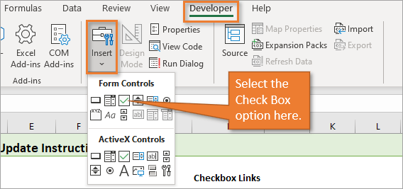
Start by going to the Developer tab on the Ribbon. If you don't see a Developer tab, it just means you need to enable it, which is easy. Here's how: Enable the Developer Tab in Excel. On this tab, choose Insert, and then select the Check Box icon under Form Controls.

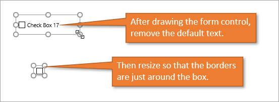
Once you've selected the form control, your cursor will look like a plus symbol, indicating that you are ready to draw your form control. Click and drag anywhere on the sheet to draw the checkbox. You'll notice that when you draw the checkbox, it comes with some default text. We want to delete that text and use text in a cell instead so that we can apply conditional formatting to it. You can also resize the form control so that it is easier to place in a cell.

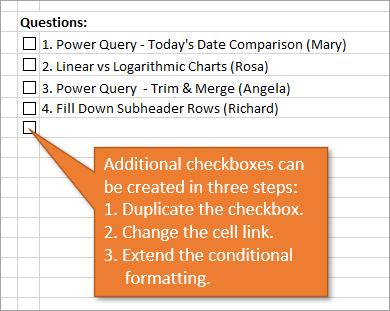
Place your checkbox in a cell and then write your task in the cell next to it. You can copy these cells down and replace the text for as many tasks as you want on your list. In the example below, I have two checkboxes for items to discuss, and four checkboxes for questions I want to answer in my meeting.

Linking the Checkbox

Now that we've created our checklist, we want to apply conditional formatting. To do this, we want to create a column of TRUE and FALSE values that we can work with. The cells in this column will show TRUE if the box for that row is checked. They will show FALSE if the box is unchecked.

We start by right-clicking on the checkbox and selecting the option that says Format Control, which will bring up the Format Control Window. On the Control tab of that window, type or select a cell from the blank column where the TRUE/FALSE value can appear. In my example, it's cell E14.

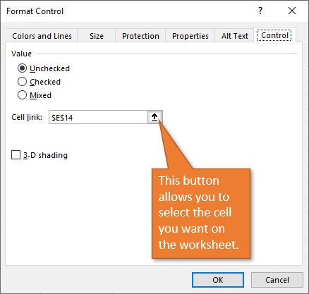
Hitting OK will close the window. Now cell E14 will return TRUE when the corresponding checkbox is checked and FALSE when it is unchecked. (The cell will appear blank until you check it for the first time.)

Applying Conditional Formatting

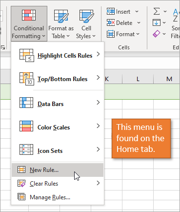
This TRUE/FALSE value column is the preliminary step to applying the conditional formatting to our task list. Now that it is in place, you can select the cell that has the name of the task. Then go to the Home tab, select Conditional Formatting, and choose New Rule.

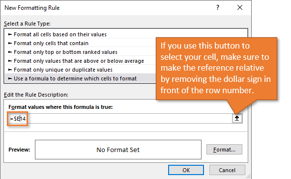
This brings up the New Formatting Rule window. Select the option that says Use a formula to determine which cells to format. The formula is simply the equal sign (=), and then the cell from the TRUE/FALSE column we created. You can either type in the cell name or choose the cell, but make sure that it is formatted as a relative reference and that no dollar symbol ($) is showing in front of the row number (a dollar symbol in front of the column number is OK). The reason we are making it a relative reference is because we intend to copy the formula down to other values in the column and we want them to correspond with the appropriate task.

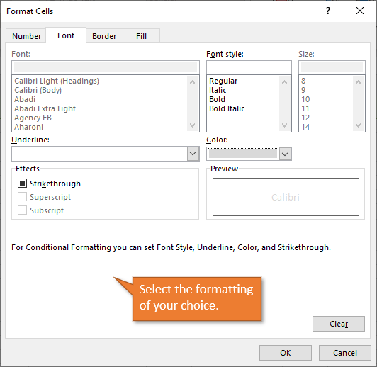
Select the Format button. Then choose whatever formatting you wish to be applied when tasks are checked off the list. This could be gray font, a grayed cell, strikethrough, or any other formatting you like.

Adding More Items to the Checklist

Now that you have created one checkbox with conditional formatting, you will likely want to add more items to the list. This is a bit of a manual process, and here are the steps.

1. Copy the checkbox and paste it to the cell below.
2. Because you've copied and pasted the checkbox, all of the new checkboxes you make will still be linked to the original cell (E14). You need to change the link for your new checkboxes to correspond to their appropriate cells (E15, E16, etc.). Right-click the checkbox, choose Format Control, and update the Cell link to the new cell.
3. The conditional formatting should automatically copy down to new rows. If it doesn't because you are on an older version of Excel, you can adjust the range for the rule in the Conditional Formatting Rule Manager to include your new task items. Here is a tutorial that explains this process in more detail: How to Apply Conditional Formatting to Rows Based on Cell Value

Tips for Modifying the Checkboxes

Here are a few tips for working with the checkbox Form Controls.

• To select the checkbox for editing, you will need to hold down Ctrl as you select it. Otherwise, when you try to click on it to copy it, you will simply be checking or unchecking the box. You can also right-click the checkbox to select it. Once the control/shape is selected, you can resize it and modify the text.
• After pasting the checkbox, you can move it using your cursor, the keyboard arrows, or by using the Align options on the Format tab of the Ribbon.
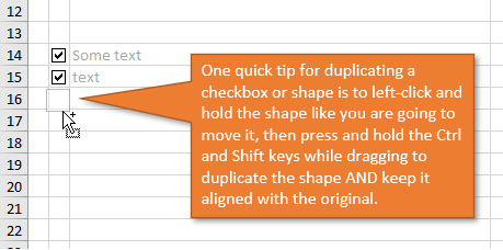
• Another tip for copying the checkbox is to first click and hold the checkbox like you are going to move it, then hold the Ctrl and Shift keys while dragging the checkbox down. This will make a duplicate copy of the shape AND keep it aligned with the original checkbox. Release the mouse button before releasing Ctrl and Shift. Check out this post on How to Copy and Align Charts and Shapes in Excel Dashbords to learn more about this shortcut.

Multiple Rules

In addition to graying out or drawing a line through completed tasks, you may want to highlight the current task in some way so that it stands out. You could change the cell color or the font color, or bold it or capitalize it—whatever you prefer to indicate that this item is what you should be focusing on.

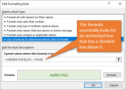
To make this kind of list, you can follow the same process as above, but this time we will add a second rule. To do this, go to the Conditional Formatting Rule Manager (Home tab> Conditional Formatting> Manage Rules) and select New Rule. We'll again use a formula to determine which cells to format, but this time, we will use an AND formula.

The AND formula will look at two criteria: 1) if the value in question is false (because the box is unchecked) AND 2) if the value above it is not false (because its checkbox is checked). If both of these are true, then the conditional formatting of your choice will be applied. Here is the formula:

This type of formatting is best for longer lists that are intended to be checked in sequential order, such as instructions or schedules. For random lists that are completed out of order, the previous formatting might be a better choice. (For example, if you had a random list of household chores to do, and you finished items 1 and 9, this formatting would highlight items 2 and 10 as the ones to focus on next, even though the order probably doesn't matter.)

Here's another tutorial you might find helpful because it goes into more detail for explaining the AND formula for multiple criteria in the formatting rule:

• Highlight Rows Between Two Dates with Conditional Formatting in Excel

Macro to Add Multiple Checkboxes

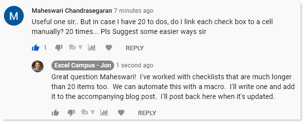
What if we need 20 (or more) checkboxes for a list? Do we have to add and link each one manually? This was a great question from Maheswari on the YouTube video.

Fortunately, we can automate this process with a VBA macro. I wrote two different macros.

Link Existing Checkboxes Macro

The first macro will create the linked cells for all existing checkboxes on the sheet. This is great if you already have a sheet with checkboxes, and want to add the conditional formatting technique to it.

Sub Link_Existing_Checkboxes()

Dim shp As Shape
Dim iCol As Long

  '# of columns to the right of the checkboxe for the linked cell
  'Use negative number to set linked cell to left of checkbox cell
  'Use 0 (zero) to link in the same cell as the checkbox
  iCol = 6
  
  'Loop through each checkbox on the existing sheet
  For Each shp In ActiveSheet.Shapes
    If shp.Type = msoFormControl And shp.FormControlType = xlCheckBox Then
      
      'Set the linked cell property to a cell to the right (or left) in the same row
      shp.OLEFormat.Object.LinkedCell = shp.TopLeftCell.Offset(, iCol).Address
      
    End If
  Next shp
  
End Sub

Create Checkboxes and Links Macro

The second macro will create a checkbox in each cell of the selected range and also setup the linked cell in a column to the right/left or same cell.

To run this macro you will first select a range of cells on the sheet where you want to add checkboxes, then run the macro.

Sub Create_Checkboxes_and_Links()

Dim c As Range
Dim shp As CheckBox
Dim iCol As Long

  '# of columns to the right of the checkboxe for the linked cell
  'Use negative number to set linked cell to left of checkbox cell
  'Use 0 (zero) to link in the same cell as the checkbox
  iCol = 7

  'Loop through each checkbox on the existing sheet
  For Each c In Selection.Cells
    
    'Create the checkbox and resize to the cell in the loop.
    Set shp = ActiveSheet.CheckBoxes.Add(c.Left, c.Top, c.Width, c.Height)
    
    With shp
      'Clear the text/description
      .Text = ""
      
      'Reset the width after the text is cleared
      .Width = c.Width
      
      'Link to cell in same row and column to right/left or same cell
      .LinkedCell = c.Offset(, iCol).Address
      
    End With
  Next c

End

Conclusion

I hope learning about these techniques proves helpful for creating lists and agendas. If you have questions, as always they are welcome in the comments. See you next time!