How to Fix an Excel Table That’s Slow to Scroll or Respond

Bottom Line: Learn how to fix an issue with using whole column references with Excel Tables that makes them slow to respond.

Skill Level: Beginner

Watch the Tutorial

Download the Excel File

If you'd like a copy of the file I use in the video, you can download it here:

Fixing Slow Response with Excel Tables

If you are working with an Excel Table and you notice a lag when you are scrolling up and down or when you move from sheet to sheet within the workbook, your problem may be whole column references. What is a whole column reference? I'll show you as I walk you through a mistake I made the other day when creating a table.

As I explain, I'll punctuate my story with some Excel tips (★) that I'm sure you'll find useful. Here goes:

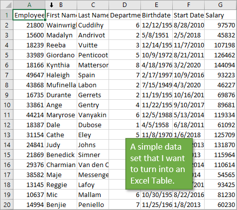
Once upon a time, I was creating a table for my Excel Campus friends to enjoy. I copied some data from another sheet and pasted it into a new sheet. It was a relatively simple data set: 7 columns wide by 250 rows deep, with no formulas. It looked like this:

The first thing I wanted to do was make my columns bigger so that I could read the data. To do this I used a trick for expanding multiple columns at the same time.

★ Excel Tip: Autofit Multiple Columns Simultaneously

If you've ever spent time adjusting each column width manually by dragging the column border left or right, then you'll appreciate this shortcut.

Excel has an autofit feature which expands your column to the exact length of the widest text in that column. You simply have to double-click on the column border (the gridline separating it from the next column) within the column's header. As you hover over that border line, your cursor changes to a line with two arrows pointing left and right.

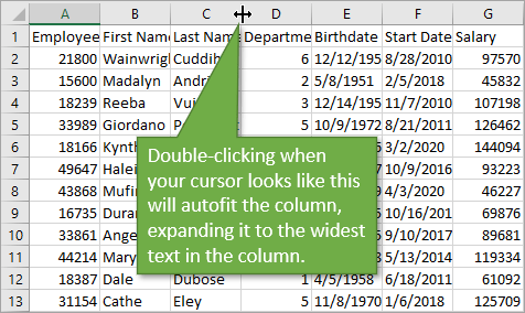
To autofit multiple columns simultaneously, you simply need to select multiple columns before double-clicking on any of the column borders within your selection.

To select multiple columns you can click on a column header and drag your cursor across multiple column headers. Or you can click on a column header and then hold down Shift or Ctrl while selecting more column headers. (Shift for contiguous columns, Ctrl for non-contiguous columns.) You'll know the columns are selected because the color of the header is different.

Once your desired columns are selected, just double-click on any one of the column borders to auto-expand all of them.

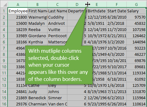
So I autofit all seven columns simultaneously and moved on to my next step, which was to turn the data into an Excel table.

★ Excel Tip: Create an Excel Table Out of Raw Data

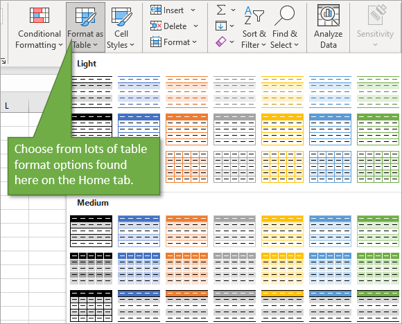
Making a table is super easy. When you have a block of data of any size, you can simply click on any cell in the data and then go to Format as Table on the Home tab. That gives you a wide selection of table formats and color schemes to choose from.

There are tons of benefits to using Excel Tables, and I outline several of them in this post: Excel Tables Tutorial Video – Beginners Guide.

I chose a light gray color style and it instantly converted my data into a table. But here is where I made my mistake. Instead of clicking on a cell anywhere in my data set before beginning, I started making my table while those 7 columns were still highlighted. Therefore my table was referencing the entire columns instead of just the cells that contained values.

The mistake isn't obvious to detect just by looking at the table. But I began to notice that when I started to scroll down, the scrolling was choppy and delayed. There was lag. This was true using the scroll wheel on the mouse as well as the with the cursor on the scroll bar. There was also a slight delay when I moved between sheets in my workbook.

★ Excel Tip: A Small Vertical Scroll Bar is a Red Flag

In addition to the lag time, one thing that might clue you in to a situation like this is a small vertical scroll bar. The more rows that you have in your data, the smaller the scroll bar appears. You can see what I mean in this comparison image.

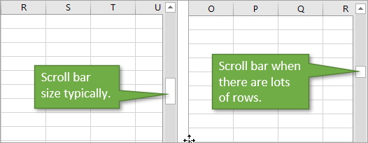
When you notice that your scroll bar is small like that, you may have a stray cell with a value or character in it way down in your sheet somewhere that can cause some performance issues. Keep in mind, however, when you save the file, the scroll bar will appear normally again.

Fixing the Issue

Once you've determined that whole column references are slowing performance for your worksheet, fixing it is pretty simple. Start by clicking anywhere in the data set. Then select the Resize Table option on the Table Design tab. That will open a Resize Table window. You can see that it is currently referencing whole columns.

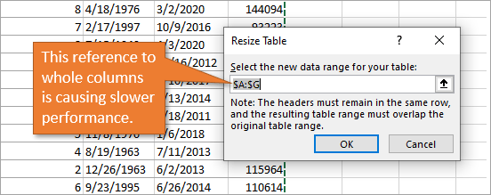
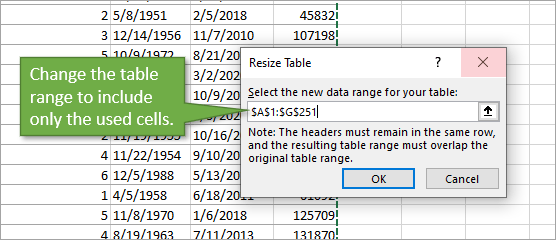
Simply change the referenced range to be the block of used cells instead of the entire columns.

★ Excel Tip: Quickly Select an Entire Block of Data

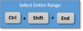
To select all of the cells in a used range, start by selecting the top leftmost cell in the range and then use the keyboard shortcut Ctrl + Shift + End.

With your table resized to include only the used cells instead of the entire columns, you'll notice improved performance right away. The lag disappears, scrolling is smooth, and you can quickly jump from sheet to sheet.

Conclusion

So, when creating tables, be sure to start by clicking on a single cell anywhere within your data set. Then Excel will automatically detect the used range. I hope that my mistake has been a useful learning experience for you! If you have any questions or comments, feel free to voice them below.