

Excel has been around for over 40 years, and in that time it has quietly accumulated a ton of features that feel hidden or forgotten. Most of them are sitting right in front of you, but they require a specific click or right-click that nobody ever thinks to try.
In this post, we're covering 19 of those hidden clicks across the ribbon, the grid, the formula bar, the status bar, and pivot tables. Each one is a small move that can save you real time on everyday tasks.
Download the Excel File and PDF guide
Complete the form below to instantly access the Excel file and PDF guide.
Video Tutorial
Watch on YouTube & Subscribe to our Channel
Ribbon Tips
1. Hide the Ribbon
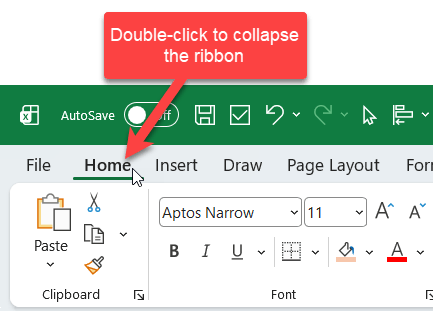
Double-click any ribbon tab to collapse the ribbon and free up vertical screen space. Click the tab once to temporarily peek at it, then click away to hide it again. Double-click to dock it back in place.
2. Ribbon Dialog Buttons
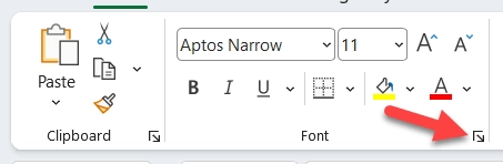
Those tiny arrow icons in the corner of each ribbon group are actually buttons. Clicking them opens dialog boxes like Format Cells, Page Setup, and more. The most useful ones live on the Home tab, but the Page Layout tab has a handy Page Setup launcher for print settings.
3. Add Buttons to the Quick Access Toolbar
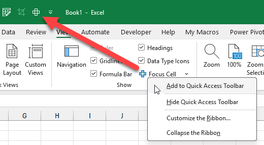
If there's a button you use often on a tab you don't visit much, right-click it and choose “Add to Quick Access Toolbar.” It will then appear at the top of the screen regardless of which tab you're on, ready for a single click any time.
Grid and Formula Tips
4. Autofit All Columns at Once
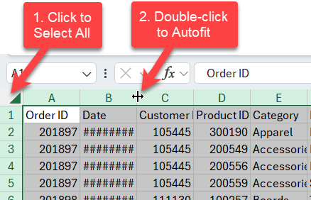
Click the triangle in the top-left corner of the grid to select all cells. Then hover between any two column headers until you see the resize cursor and double-click. Every column on the sheet autofits instantly.
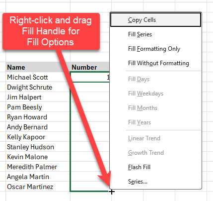
5. Fill Handle Options
Most people know you can left-click and drag the fill handle to copy a value down. But if you right-click and drag instead, Excel automatically opens a menu when you release the button. From there you can choose Copy Cells, Fill Series, Fill Formatting Only, and more.
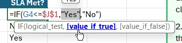
6. Function ScreenTip Links
While editing a formula, the screentip shows the function signature below the cell. You can click the function name to open its Excel help page. Hover over any argument name to select all the text for that argument, which is much faster than manually selecting it, especially on a laptop trackpad.
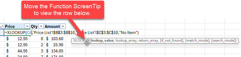
7. Move the Function ScreenTip
The screentip can block the row below the formula you're editing. Just hover over the border of the screentip, left-click and hold, then drag it out of the way. This works on Windows, Mac, and the Web version.
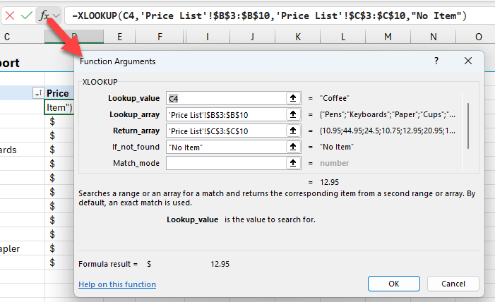
8. Function Arguments Window
Click the fx button next to the formula bar to open the Function Arguments window. It lists every argument for the active function. Click inside any argument field and a plain-English description appears at the bottom, which is a great way to understand a function you haven't used before.
9. Expand the Formula Bar
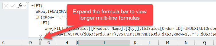
Long or multi-line formulas often look cut off in the default formula bar. Hover over the bottom border of the formula bar until you see a double arrow, then drag it down to reveal the full formula. Use Ctrl+Shift+U to toggle it quickly.
Status Bar Tips
10. Sheet Activate Window
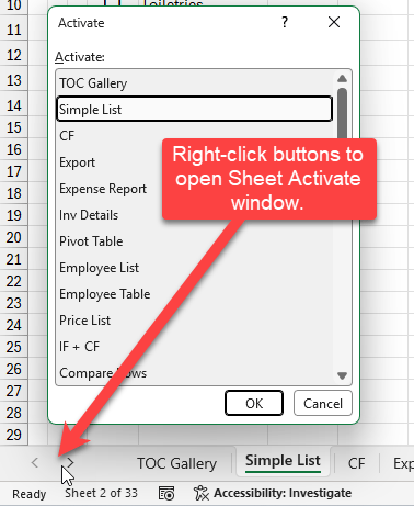
When a workbook has dozens of tabs, scrolling through them is painful. Right-click either of the sheet navigation arrows in the bottom-left corner to open the Activate window, which shows a vertical scrollable list of every sheet. Double-click any sheet name to jump there instantly.
11. Navigation Pane
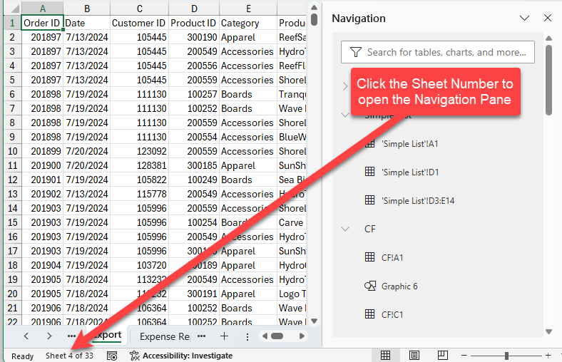
On Microsoft 365, click the sheet count number next to the navigation arrows to open the Navigation Pane. It lists all sheets plus every table, pivot table, and chart inside each one. Click any object to navigate directly to it.
12. Copy Status Bar Stats
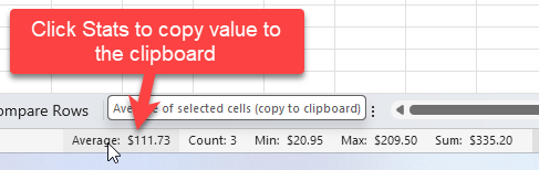
When you select a range of numbers, the status bar shows stats like Sum, Average, and Count. Left-click any of those stats to copy that value straight to your clipboard. It pastes as a hard-coded number, but it's great for quick reconciliations.
13. Enable Stats
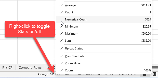
If your status bar isn't showing the stats you need, right-click anywhere on it to open the Customize Status Bar menu. Toggle any stat on or off with a single click.
14. Zoom Dialog
Click the zoom percentage in the bottom-right corner to open the Zoom dialog. Choose a preset level and double-click it to apply and close in one move. To jump back to 100% with a keyboard shortcut, press Alt, W, J.
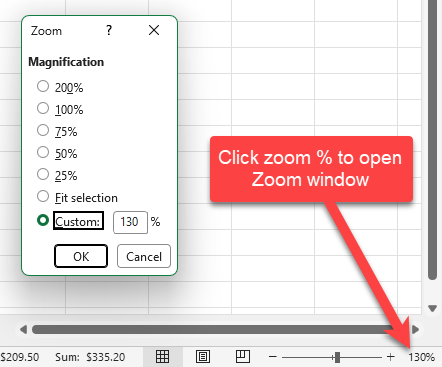
Bonus tip: Double-click any of the items in the window apply them and close the window, so you don't have to click the OK button.
15. Restore Scroll Bar Size
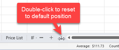
If the horizontal scroll bar has been resized to show more sheet tabs, you can double-click the resize handle to snap it back to its default width. The same trick works on the Name Box if you've accidentally made it wider than you want.
Tables and Pivot Table Tips
16. Apply and Clear Table Formatting
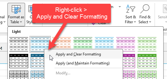
When you apply a table style over existing cell formatting, the results often look messy. Instead of left-clicking the style, right-click it and choose “Apply and Clear Formatting.” This strips any existing manual formatting and applies the table style cleanly.
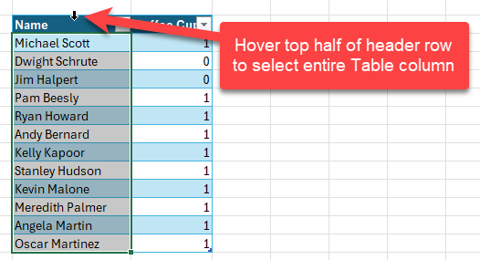
17. Select a Table Column
When writing formulas that reference an Excel Table, hover over the top half of a column header until the cursor turns into a down arrow, then click. This inserts a structured reference to that entire table column automatically.
Here's an example using the FILTER function with a table column reference:
A quick look at the FILTER function before we dive in. It returns a filtered subset of a range based on a condition you define. The function arguments are:
- array: the range or table column to return values from
- include: a boolean array the same height as array that determines which rows to keep
- if_empty: value to return if no rows match the condition (optional)
=FILTER(Table1[Name],Table1[Coffee Cups]=0)
18. Expand and Collapse Pivot Fields
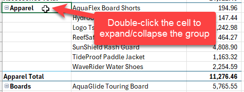
Pivot tables show small expand and collapse buttons next to grouped row items. Those tiny buttons can be hard to click, especially when zoomed out. Just double-click anywhere on the row label itself to expand or collapse it.
19. Pivot Table Classic Layout
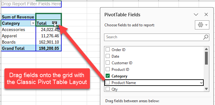
Right-click a pivot table, go to PivotTable Options, click the Display tab, and check “Classic PivotTable layout.” This switches to the older-style layout where you can drag fields directly onto the grid, making it faster to build and rearrange the report on the fly.
Summary
Excel's best-kept secrets are often just one unexpected click away. From collapsing the ribbon to free up screen space, to right-clicking the fill handle for smarter fill options, to double-clicking pivot row labels to expand groups without fumbling for tiny buttons, each of these 19 features takes seconds to learn and pays off every time you use it. Download the free PDF guide linked below to keep this list handy, and let us know in the comments which one was new to you.


I would like to thank you and your team. Your videos made my job easier and dynamic, the time I save to complete tasks is immense. I’m 64, until 5 years ago I was working as a cook until, do to injury, I couldn’t work for months. If was then that I wanted to learn how to use Excel and Word and I began to watch your videos to help me, because you explain everything so clearly and effectively . Now I work in an office and, modestly aside, I’m the office hero, the go to person. Thank you John, in my view you are amongst those who makes this world a better place.