Why Table Number Formatting Doesn’t Copy Down and How to Fix It

Bottom line: Learn why the number formatting for new rows of a table doesn't always get copied down and how to fix it.

Skill level: Beginner

Video Tutorial

Number Formatting Not Copying Down

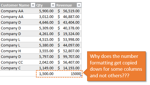
I stumbled on some weird table behavior recently and had to investigate.  When adding new data to the bottom of my table, the number formatting from the cell above wasn't getting copied down.

All of the cells in the column had the same number formatting applied, so I expected the cells below in the new row to inherit the number format.  However, that wasn't the case.

All Cells in the Column Must Be Formatted at the Same Time

The reason this happens is because the number formatting was NOT applied to all of the cells in the column at the same time.

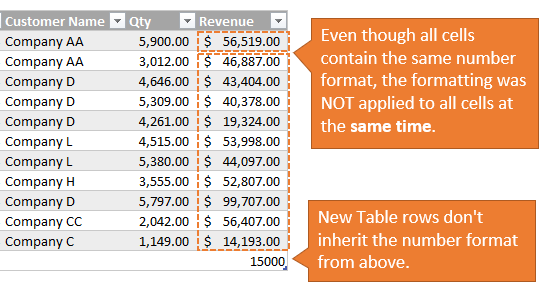
If you apply number formatting to one cell, then apply the same format to the rest of the cells in the column later, the Table does NOT set that as the formatting for the entire column.  So, we don't get the same formatting copied down for new rows.

There is no way that I've found to check if a number format has been applied to all cells in the column at the same time, so it is a bit confusing.

How to Fix It

The solution is pretty simple here.  We just have to apply the number formatting to all cells in the column at the SAME TIME.

This can be a time consuming task if your Table has a lot of columns, so I want to share two ways to make this process easier.

Tip #1: Shortcuts to Select Entire Table Columns

The first tip is pretty simple and really requires two steps.

1. Select all of the cells in the column.
2. Re-apply the number formatting.

How to Select All Cells in a Table Column

If your Table has a lot of rows, this task can be time consuming.  Here are two shortcuts to select all cells in the data body range of the column.  The data body range is the range of cells below the Table header and above the Total Row.

Use the Mouse

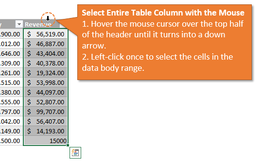
To select all the cells in the column with the mouse:

1. Hover the mouse cursor over the top half of the header cell until the cursor turns into a down arrow.
2. Left-click once to select all cells in the data body range.

Use a Keyboard Shortcut

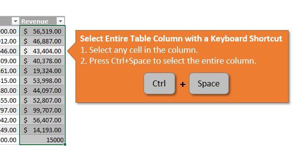
The keyboard shortcut to select a Table column is Ctrl+Space.

1. Select any cell inside the column.
2. Press Ctrl+Space to select all cells in the data body range.

Checkout my other articles on 5 Keyboard Shortcuts for Rows and Columns and 2 Keyboard Shortcuts to Select Columns with Blank Cells to learn some additional tips.

Apply the Number Formatting

After the cells are selected, apply the number formatting to the entire column.  This will set the number formatting for the column and all new rows should inherit the column's number format.

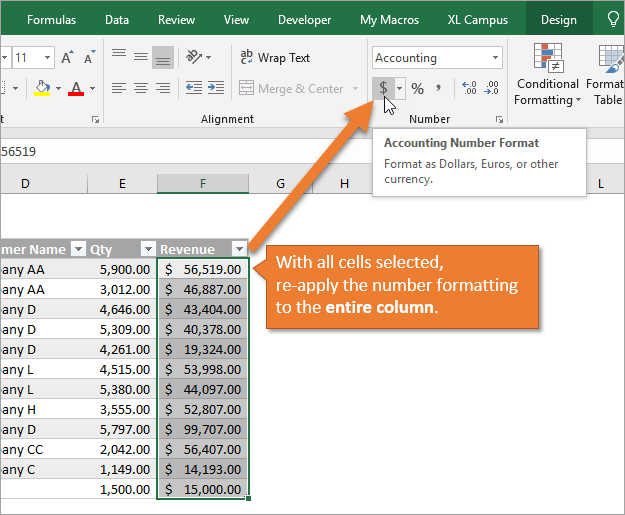
Important Note: If you are using the Format Cells window to re-apply number formatting, then you might have to first change the number format to a different format, then change it back to your original format.  The Format Cells window does NOT reset the formatting for the entire column if all the cells in the column already contain that number format.  See the video above for more details.

Tip #2: Table Number Formatting Macro

If your Table has a lot of columns, or your workbook has a lot of Tables, then this task could take a long time to do manually.  So I wrote a few macros that automate the process.

You can download the file that contains the VBA code.

I explain how these macros work in the video above.   So make sure to watch it if you are going to use the macros in your projects.

Macro #1: Fix All Columns in a Specific Table

The first macro loops through all of the columns in a Table and sets the number formatting for the entire column.  It uses the number formatting from the first cell in the column as the basis.  However, you can change the code to use the cell in the last row of the column instead.

Sub Table_Number_Formatting()
'Copy number formatting down each table column
'Source: https://www.excelcampus.com/tables/table-number-formatting/

Dim lo As ListObject
Dim lc As ListColumn

  'Set a reference to a table
  Set lo = ActiveSheet.ListObjects(1)
  'Set lo = ThisWorkbook.Worksheets("Data").ListObjects("Table1")
  
  'Loop through all list columns in the table
  For Each lc In lo.ListColumns
    'Set the number formatting of the entire column to the number formatting in the first row
    lc.DataBodyRange.NumberFormat = lc.DataBodyRange(1, 1).NumberFormat
  Next lc

End Sub

Macro #2: Fix All Columns in the Selected Table

This macro will run on the Table the user has selected.  Just select a cell inside a Table before running it.

Sub Table_Number_Formatting_Selected_Table()
'Copy number formatting down each table column on the selected table.
'Source: https://www.excelcampus.com/tables/table-number-formatting/

Dim lo As ListObject
Dim lc As ListColumn

  'Set a reference to the selected table
  On Error Resume Next
    Set lo = Selection.ListObject
  On Error GoTo 0
  
  'If a table is selected then format it
  If Not lo Is Nothing Then
    
    'Loop through all list columns in the table
    For Each lc In lo.ListColumns
      'Set the number formatting of the entire column to the number formatting in the first row
      lc.DataBodyRange.NumberFormat = lc.DataBodyRange(1, 1).NumberFormat
      
      'Use the line below to set it to the last row in the table
      'lc.DataBodyRange.NumberFormat = lc.DataBodyRange(lo.DataBodyRange.Rows.Count, 1).NumberFormat
    Next lc
    
  Else 'Cell in table not selected
    MsgBox "Please select a cell inside a Table first.", vbOKOnly, "Table Formatting Macro"
  End If
  
End Sub

Macro #3: Fix All Tables in the Workbook

The Table_Number_Formatting_All_Tables macro will fix the number formatting in all Tables in a workbook.  It loops through each sheet in the workbook, then loops through all tables on the sheet, and finally loops through all columns in each Table.

This is nice if you have a workbook with a lot of Tables and want to make sure you or your users don't run into this formatting issue.

Sub Table_Number_Formatting_All_Tables()
'Copy number formatting down each entire table column
'For each table in the workbook
'Source: https://www.excelcampus.com/tables/table-number-formatting/

Dim lo As ListObject
Dim lc As ListColumn
Dim ws As Worksheet

  'Loop through each sheet in the active workbook
  For Each ws In ActiveWorkbook.Worksheets
    'Loop through all tables on the sheet
    For Each lo In ws.ListObjects
      'Loop through all list columns in the table
      For Each lc In lo.ListColumns
        'Set the number formatting of the entire column to the number formatting in the first row
        lc.DataBodyRange.NumberFormat = lc.DataBodyRange(1, 1).NumberFormat
        
        'Use the line below to set it to the last row in the table
        'lc.DataBodyRange.NumberFormat = lc.DataBodyRange(lo.DataBodyRange.Rows.Count, 1).NumberFormat
      Next lc
    Next lo
  Next ws
  
  MsgBox "Number Formatting has been updated for all Tables in the active workbook.", vbOKOnly, "Table Number Formatting Macro"

End Sub

The Macros ONLY Change Number Formatting

It's important to note that these macros will apply the Number Formatting to all cells in the column for EACH column.  If you have some columns with mixed number formatting, then you might want to go with the manual approach explained in Tip #1.

The macro is ONLY applying number formatting.  It will NOT change any other formatting properties like font/fill color, borders, conditional formatting, etc.  It ONLY changes number formatting.

We can't undo the changes made by these macros, so make sure to save a backup copy first.

We could also modify the macro to only run on columns that contain numbers, dates, or even specific number formats.  Please leave a comment below if you are interested in that and I will share some code.

Add the Macros to Your Personal Macro Workbook

Any of these macros can be added to your Personal Macro Workbook to run on any open Excel file.  You can also add a macro button to the ribbon to make it easy to run the macro at any time.

Checkout my 4-part video series on the Personal Macro Workbook to learn how to set this up.

Is this behavior a bug?

What do you think about this behavior?  My initial thought is that if all the cells in the column have the same formatting, any new cells should inherit that same formatting, even if formatting is not applied at the same time.

I can see that we might not want that behavior if there are different number formats used in the column.  However, if the entire column has the same number format, then it makes sense that any new Table rows will inherit the formatting from above.

Are there any cases where you wouldn't want this to happen?  If so, please leave a comment below.  Thank you! 🙂