Bottom line: Learn how to change the date formatting for a grouped field in a pivot table.
Skill level: Intermediate
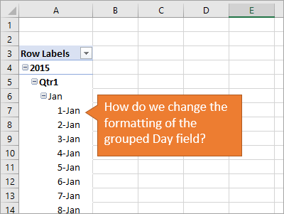
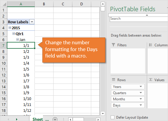
Changing the Days Field Number Formatting Doesn't Work
When we group a Date field in a pivot table using the Group feature, the number formatting for the Day field is fixed. It has the following format “Day-Month” or “d-mmm”.
If we try to change the number format of the Day/Date field it does not work. Nothing changes when we go to Field Settings > Number Format, and change the number format to a custom or date format.
Why?
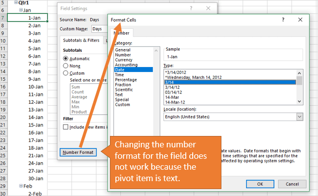
The number formatting does not work because the pivot item is actually text, NOT a date.
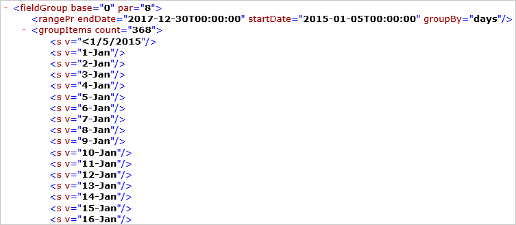
When we group the fields, the group feature creates a Days item for each day of a single year. It keeps the month name in the Day field names, and this is actually a grouping of day numbers (1-31) for each month.
We can actually see this list of text items in the pivotCacheDefinition.xml file. To see that you can change the file extension of the Excel file to .zip, and navigate to the PivotCache folder.
Since these are text items that represent the days of the year, we won't be able to change the number formatting of the cells directly in Excel. However, there are a few workarounds.
Solution #1 – Don't Use Date Groups
The first solution is to create fields (columns) in the source data range with the various groups for Year, Quarter, Month, Days, etc. I explain this in detail in my article on Grouping Dates in a Pivot Table VERSUS Grouping Dates in the Source Data.

Using your own fields from the source data for the different date groups will give you control over the number formatting of the field in the pivot table.
You can also create a Calendar Table with the groupings if you are using Power Pivot.
Automatic Date Field Grouping
If you are using Excel 2016 (Office 365) then the date field is automatically grouped when you add it to the pivot table.
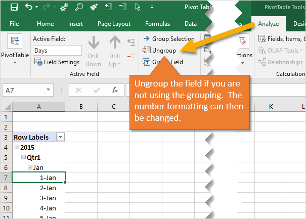
To Ungroup the date field:
- Select a cell inside the pivot table in one of the date fields.
- Press the Ungroup button on the Analyze tab of the ribbon.
The automatic grouping is a default setting that can be changed. See my article on Grouping Dates in a Pivot Table VERSUS Grouping Dates in the Source Data to learn more.
Once the date field is Ungrouped you can change the number formatting of the field.
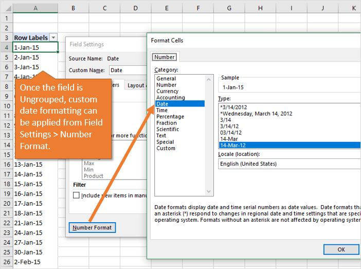
To change the number formatting on the ungrouped Date field:
- Right-click a cell in the date field of the pivot table.
- Choose Field Settings…
- Click the Number Format button.
- Change the Date formatting in the Format Cells window.
- Press OK and OK.
Again, this only works on fields that are NOT grouped. If you group the field again after changing the formatting, the formatting for the items in the Days field will change back to “1-Jan”.
Solution #2 – Change the Pivot Item Names with VBA
If you really want to use the Group Field feature, then we can use a macro to change the pivot item names. This will make it look like the date formatting has changed, but we are actually changing the text in each pivot item name.
The following macro will loop through all the pivot items of the grouped Days field, and change the number formatting to a custom format. By default I set it to “m/d”, but you can change this to any date format for the month and day. Just remember that the item is NOT going to contain the year, since the item is not an actual date.
Download the File
Download the Excel file that contains the macro.
The Change Days Field Formatting Macro
Sub Change_Days_Field_Formatting()
'Change the number formatting of the Days field
'for Grouped pivot table date field.
'Source: https://www.excelcampus.com/pivot-tables/grouped-date-field-formatting/

Dim pt As PivotTable
Dim pi As PivotItem


'IMPORTANT: Change the following to the name of the
'grouped Days field.  This is usually Days or the name
'of your date field.

Const sDaysField As String = "Days"

  'Set reference to the first pivot table on the sheet
  'This can be changed to reference a pivot table name
  'Set pt = ActiveSheet.PivotTables("PivotTable1")

  Set pt = ActiveSheet.PivotTables(1)

  'Set the names back to their default source name
  For Each pi In pt.PivotFields(sDaysField).PivotItems
    'Bypasses the first and last items "<1/1/2015"...
    If Left(pi.Name, 1) <> "<" And Left(pi.Name, 1) <> ">" Then
      pi.Name = pi.SourceName
    End If
  Next pi

  'Set the names to a custom number format
  For Each pi In pt.PivotFields(sDaysField).PivotItems
    If Left(pi.Name, 1) <> "<" And Left(pi.Name, 1) <> ">" Then
      'Change the "m/d" format below to a custom number format.
      'Year 2020 is used for leap year.
      pi.Name = Format(DateValue(pi.SourceName & "-2020"), "m/d")
    End If
  Next pi

End Sub
How the Macro Works
The macro first loops the pivot items in the Days field to restore the pivot item name to it's default source name. Two different pivot items cannot have the same name. So this should prevent any errors when changing or trying different formats.
The second loop changes each pivot item to the new format. It uses the DateValue function to change the pivot item name “1-Jan” to a date. It then uses the Format function to change the formatting of the date to text. By default it uses the “m/d” format. This can be changed to another format with the month and day. Each item must be unique, so you will want to use both the month and day in the item name.
You could probably separate this macro into two macros, and only run the first reset loop as needed. The macro takes about 15 seconds to run on my computer because of all the looping. But it's not one you will have to run often.
It's also important to mention that this is running on the pivot items, not the pivot cache. So the newly named items will only be changed on the pivot table you run the macro on.
Change Grouped Items Number Formatting Macro
Natilia asked a great question in the comments below about changing the number formatting for grouped numbers. This is the same issue as the date groups. The group names are text, not numbers. However, we can use a macro to change these as well.
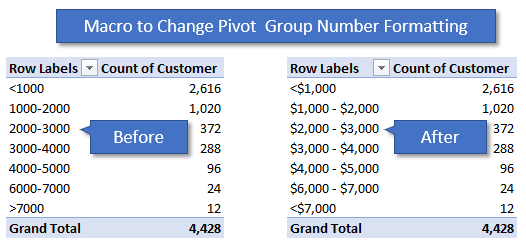
Here is the macro code. You will just need to change the value of the sGroupField constant at the top to the name of your grouped field. You can also change the number format in the sNumberFormat if needed.
Sub Change_Grouped_Field_Number_Formatting()
'Change the number formatting of the grouped number field
'Source: https://www.excelcampus.com/pivot-tables/grouped-date-field-formatting/

Dim pt As PivotTable
Dim pi As PivotItem
Dim sGroup() As String
Dim sGroupName As String


'IMPORTANT: Change the following to the name of the
'grouped number field in the rows or columns area.

Const sGroupedField As String = "Quantity"
Const sNumberFormat As String = "$#,###"

  'Set reference to the first pivot table on the sheet
  'This can be changed to reference a pivot table name
  'Set pt = ActiveSheet.PivotTables("PivotTable1")

  Set pt = ActiveSheet.PivotTables(1)

  'Set the names back to their default source name
  For Each pi In pt.PivotFields(sGroupedField).PivotItems
    'Bypasses the first and last items "<1/1/2015"...
    If Left(pi.Name, 1) <> "<" And Left(pi.Name, 1) <> ">" Then
      pi.Name = pi.SourceName
    End If
  Next pi

  'Set the names to a custom number format
  For Each pi In pt.PivotFields(sGroupedField).PivotItems

    If Left(pi.Name, 1) = "<" Or Left(pi.Name, 1) = ">" Then
      sGroupName = "<" & Format(Mid(pi.Name, 2, Len(pi.Name)), sNumberFormat)
    Else
      sGroup = Split(pi.Name, "-")
      sGroupName = Format(sGroup(0), sNumberFormat) & " - " & Format(sGroup(1), sNumberFormat)
    End If

    If sGroupName <> "" Then pi.Name = sGroupName

  Next pi

End Sub
Final Verdict
I hope you find that helpful. I would suggest going with Solution #1 unless you really want to use the Group feature.
Please leave a comment below with any questions or suggestions on how we can improve this. Thanks so much! 🙂


John, could you send the XL file that goes with this article? That way I can try out your suggestions and follow-up if there are issues or questions. Thanks. Mark
Hi Mark,
Sure thing! I added the file to the download section in the article above. Thanks! 🙂
Thanks Jon, ungrouping works perfectly. Thanks for sharing
This is definitely a data pet peeve of mine. I tend to go the first option of adding fields to the source data after going crazy trying to reformat the group dates. At least I have better control of that. Thanks for the options, I’ll explore those when I have data and time.
Thanks Dave! Yeah it’s just good to be aware of the issue that we can’t direct change the date format. Have a nice weekend! 🙂
hello Jon.. i had a issue of pivot picking up the month instead of dd/dd/yyyy format from its source data and when i clicked on grouping and ungrouping then it automatically picked the correct date format! how this is possible?
i was challenged with this last week. perfect timing – thx
HI JOHN, THANK YOU FOR YOUR INFO AND KNOWLEDGE SHARING, AND DUE TO YOUR GUIDANCE, I START LOVING EXCEL AGAIN :)))
REGRDS,
EK.
Hi Jon,
Thank you for the comprehensive post. I have a question about graphs as well. When I make a bar-line graph where I have two series ( each has a bar and line graph) so I have two lines and two bars. I need the data points of each line to be aligned with the bar of the same series ( it is always aligned in the middle between the two bars. Please tell me how to make such alignment.
Thank you in advance.
Noha
Just FYI- if you have office 365 Excel 2016 and it auto groups your dates, then ungrouping does not let you change format- there is still no number format button. It also won’t sort by date correctly no matter what you do. Idiot proofing gone wrong is so very frustrating! Version 1708 Build 8431.2153.
It works on my O365 1809 and 1802 versions (September 2018 and February 2018).
You can ungroup and immediately upon ungrouping, the date field reverts to the cell format already applied to it. I can also change the cell formatting.
You’ve lost the previously calculated fields (year/month/day) etc.
Hello Jon, can I format groups and how in Pivot Tables? I created groups and need to add number format “accounting”, so i.e. range 0-10000 will display $0-$10,000. I went to Field Settings to change number format, but my selection is not working. Thank you, Natalia
Hi Natalia,
Great question! Unfortunately it’s the same issue as the date formatting. The number groups are text. You can manually change each cell and type in the $ and commas.
We can also use a macro to save time with this process. I modified the macro above to work on number groups. In the macro below you will just need to change the value of the sGroupField constant at the top to the name of your grouped field. You can also change the number format if needed.
Try it out and let me know if you have any questions. Thanks!
I added a section in the post above with the code as well. It might take a few hours for it to clear the cache and appear there.
Hello, thank you for this post. However, when I am adding same months in my database for different categories, it is still appearing as different lines in my pivot table. What is the way out?
PLEASE YOU SAID THAT, I AM EDITING PIVOT TABLE,HOW TO AUTOMATIC CHANGE MY MAIN SHEET / DATA SHEET
PLEASE YOU SOLVED THAT, WILL EDIT THE PIVOT TABLE, HOW TO CHANGE MAIN SHEET/DATA SHEET,
IT IS POSSIBLE. PLZ REPLAY ME.
Here is a super easy solution:
– On the original data change the date field formatting to number. This will give the Excel number for that day.
– Create your pivot table and add the date as a field.
– Format the date field as a date. Excel will only see the info as a number and format it as a date.
No macros, reorganizing, or ungrouping needed.
Hope this works for you.
Hi Harry,
Very interesting solution. Thanks for sharing. I’m not sure how it solves the issue with date groups though. You won’t be able to group the field by time period (year, month, day, etc.) when the source field is a number. Therefore, you would have to create date groups with calculated columns, which is solution #1 in the article.
The other drawback is that the number format will be displayed in the filter drop-down menu and any slicers for the field.
Maybe I don’t fully understand your solution though. Thanks again!
I created a column that was =INT(date field). This truncated the date/time to only the date. Then used this calculated field in the pivot table. The pivot table allowed me to format this number as a Date. This grouped my data by days (which is what I wanted).
Thanks for all the other tips.
I can verify that this solution worked!
Found this post and I hope you are still monitoring the original question
I have Excel for Mac – these solutions work on PC however when I move to my Mac – it painfully does not….
Anyone have any experience with the silly bratty date grouping issue for Pivot tables on Mac.
The leading zeros are in the raw data and when create the pivot it loses them and moves all of my single digit dates throughout the grouped table. I have a ton of work to do every time I refresh weekly with my years worth of data….
Any thoughts are welcome! You have come the closest to any other input we have found on google.
Thanks in advance!
Awesome! I would have never got there…
Great explanations – especially the one using the macro – exactly what I needed to pretty up financial values that were bands of $10m upwards – hard to read without the commas so the macro worked a treat!!!
Hi Jon
I don’t seem to get the Number Format option in the bottom left of the Field Formatting dialog; I’m sourcing my data from a tabular cube so not sure if this makes a difference.
My dates look like this: ‘4/5/2018 11:20:00 AM’ and are displayed this way, but I just want to display the date as dd/mm/yyyy (Australian format).
I’m wondering if I’ll have to have the format specified in the data cube itself.
Any further thoughts or suggestions gratefully accepted.
Cheers, Paul
UPDATE
After writing my question, I revisited my data & cube – the field was set to be a smalldatetime field in my SQL table which set it as text for some reason in my cube.
After changing the SQL type to datetime, my cube then recognised it as a date and the pivot reflected the format as required.
(side note: the Number Format option in Field Settings still did not appear).
cheers Paul
ActiveSheet.PivotTables(1).PivotFields(1).NumberFormat = “dd mmm”
One thing I discovered today is that Excel does not appear to Support Date Groups in Pivot tables if you have used the Date Model option (normally if you want to add Distinct Counts on items in the data you are pivoting).. so you can either have distinct count with Data Model OR Grouped Dates…but NOT BOTH
Thank you very much. The ungroup worked for me.
I have a work around for the ‘text’ problem and grouping. I changed all my day/times to general > integers and copied and pasted the values into the appropriate cells – then inserted the pivot table. Afterwards the pivot table would sort by month/day/year format (which is the format I need)….or just by year…or by month etc. IDK why it works – only that it does!
It was very professional. Thank you!
My recent case – clean date data was being pasted in from Access to the Excel worksheet, which included blank date field values. The problem for me was due to using an existing Excel paste area which must have started to include empty cell markers that look like text. I deleted the area and used clean unused excel cells for the paste and this worked fine in allowing the pivot table to read the column as dates.
perfect article. thank you!
Thanks, this was the most useful piece of information I’ve found so far regarding the matter.
Perfect thanks .
Excellent, very helpful.
I came up with a little easier solution. Don’t let Excel know it’s a date. I created an additional field at the end of my table with the following formula =text([datefield],”MM/DD/YYYY”). If Excel doesn’t recognize that it is a date it won’t do the format change.
Thank you, ungroup worked out – simple and fast solution.
And very well explained – thank you for the screenshots and the technical insights.
Have a nice day!
Thanks a lot
ActiveSheet.PivotTables(1).PivotFields(1).NumberFormat = “dd mmm”
Thanks a lot, the ungroup option is exactly what I was looking for!
Hi, thank you for your explanation. my dates are chosen from a data validation. I was able to un-group the dates. but when i go to fields setting under date; I don’t have the number format?? and if I change the number format from Home, it changes in my pivot table but not in my Chart. can you please help. I need it to change in the chart. thank you so much.
“Ungroup” worked perfectly. Thanks!
Great Explanation.Thanks..
thanks, Ungroup was exactly what I needed to learn about
Very helpful! Thank you.
Thanks John. I didn’t know what excel did on the date grouping in pivot tables and it was driving me nuts – my work arounds were not as elegant as yours. Now knowing that I can ungroup easily directly in the pivot tables is fantastic. Many thanks.
Thanks for the detailed description of this issue. Helped me out a lot!
the Ungrouping Function – thank you!!
You are awesome
I created a table that groups by week, and I can’t change the source data because it’s pulling automatically from a document that other people use. Is there any way to change to format to exclude the year so that the columns aren’t so wide? (I can’t post a screenshot can I?)
Thank you John……
How can I change the name of Date grouping by Month. In normal pivots I can change this, in a data model it always defaults to Jan, Feb, March and I can’t change them.
I am thinking of adding a Month, Day, Year column to my data to avoid this issue, but my data sets are 500-800k rows so it’s not super practical to have to add this every time.
Thank you for this solution. It was exactly what I needed. (I used the ungrouping solution.)
Thanks so much. Ungrouping fixed it for me!!
Thank you for your tip on un-grouping dates in pivot tables. The answer I was looking for with a problem I was having with a pivot table I was working on
Thanks so much! This was so helpful, I was loosing my mind trying to figure out why the pivot was grouping my dates automatically.
great! the ungroupping helped 🙂 thanks
Finally fixed an issue that had been bugging me for years – could not work out why the X-Axis on one of my many pivot charts showed dates in the format dd/mm/yyyy 0:00
Needed to click on the Number Format button and pick the correct format – despite the data being dates !
Thank you for easy solution.
Going into pivot table Analyze and ungrouping worked fine. Problem solved, 365 excell.