How to Merge Tables with Power Query – Similar to Vlookup

Bottom Line: Learn how to merge tables or queries in Power Query to look up data and return matching results.  This is similar to a Vlookup or Join where a relationship is created between two tables.

Skill Level: Intermediate

Video Tutorial

Download the Excel File

You can practice merging tables using the same Excel file that I use in the video. Download it here:

Overview

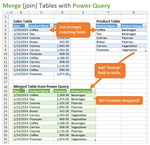
We received a great question from a member of the Excel Campus community, Bill Evans, who wanted to know how to take data from two tables that are formatted differently and combine them into a single sheet using Power Query.

The answer involves using the Merge (or join) feature in Power Query. It basically creates a relationship between two tables to look up data and return matching results.

This is similar to what a VLOOKUP can accomplish with a formula. However, Power Query allows us to automate this entire process, along with any other data cleanup work, and is less prone to formula errors.

If you are looking to combine data by stacking tables together, that is called an Append. You can learn how to append tables in this post: How to Combine Tables with Power Query.

If all of this is sounding a little over your head because you are somewhat new to Power Query, take a break from this post and head over to my Power Query Overview. That will give you a better understanding of how and why it's used. And this tutorial will walk you through installing Power Query.

Step 1: Create a Connection to the Lookup Table

To join two tables, we want to start by creating a connection-only query for the table that we will be looking up. Usually, when a query is run, it outputs the result in a new table in the workbook. But for this step, we just want to create the connection without creating a new output table. Here's how:

Go to the Power Query editor by clicking on From Table/Range on the Data or Power Query tab (depending on which version of Excel you are using).

This brings up a preview of your data. To create a connection:

1. Click on the bottom half of the Close & Load split-button.
2. Select Close & Load To…
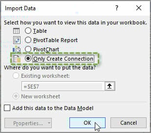
3. That brings up the Import Data window. From here, select Only Create Connection.
4. Click OK.

Step 2: Use the Merge Feature to Join the Tables

Once we've established a connection for the lookup table, we can merge it with the data from another table. This other table does not have to be in the same workbook. It could be from another workbook, a CSV file, a webpage, a database, or some other source.

In this example we will use a Table in Excel as the source.

To create a query for that source, start by going to the Data (or Power Query) tab and selecting From Table/Range.

On the Home tab of the Ribbon, select Merge Queries. This brings up the Merge window.

1. First, in the top part, you can select the column that you want to use for merging.
2. Then, in the middle, you select the table that you want to merge your data into.
3. Finally, in the lower section, you will choose the matching column. For my example the columns that we are using to merge both contain the customer ID numbers.

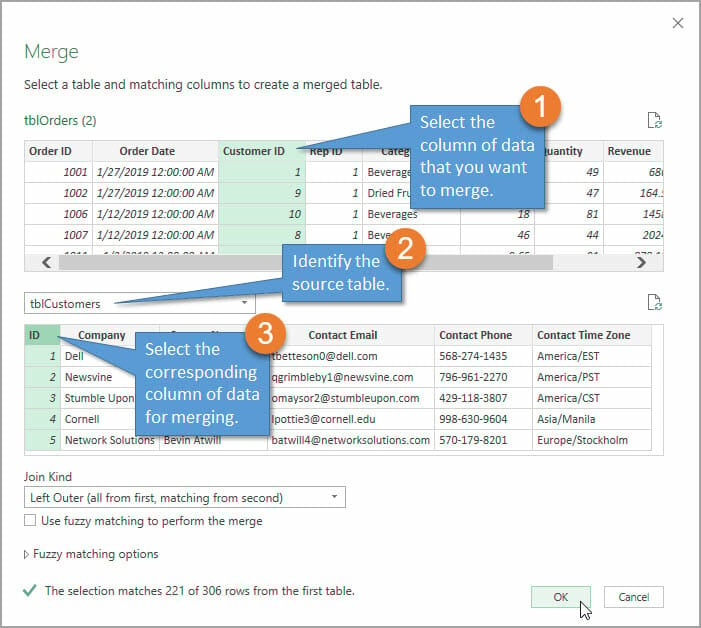
You can leave the Join Kind field as Left Outer. The Left Outer join will return all of the rows from the first table, and only the matching rows from the second table.

At the bottom of the window you'll see the numbers of rows that were matched. In this case it says “The selection matches 221 of 306 rows from the first table.” This means that some rows from the orders table did not have a matching ID in the customers table. It's ok for now and we'll look at how to fix it below.

We can go ahead and press OK.

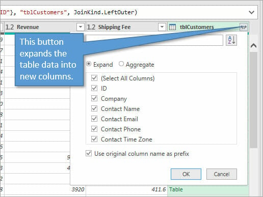
This adds a new column to your query, which can be expanded to include any of the columns from the source table. By clicking on the Expand button, you can select which columns to include.

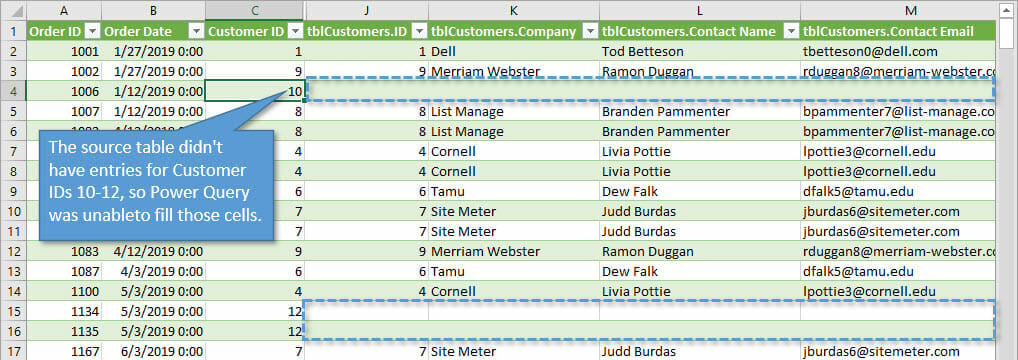
You may notice that some of the tables have rows that say “null” and when you close and load your query, those cells are blank. This is because when you merged the two tables, Power Query was unable to find some of the data in the source table.

You'll notice that all of the new columns have headers that begin with the name of the table it came from. That can get a little annoying, so if you want to avoid that, just uncheck the box that says Use original column name as prefix.

Updating the Data

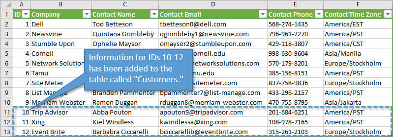
In order to fix the null entries, you can just add the appropriate rows to the lookup table, and then refresh the query.

You can refresh the query by right-clicking anywhere on the table and selecting Refresh or by using the Refresh All button on the Data tab of the Ribbon. That will rerun the steps of the query and fill in the new data.

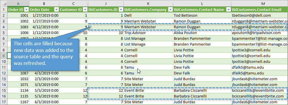
Going forward, if you make any additions or deletions to the source table(s), a simple refresh of the query will instantly update the output table.

Free Training Webinar on the Power Tools

Right now I'm running a free training webinar on all of the Power Tools in Excel. This includes Power Query, Power Pivot, Power BI, pivot tables, macros & VBA, and more.

It's called The Modern Excel Blueprint. During the webinar I explain what these tools are and how they can fit into your workflow.

You will also learn how to become the Excel Hero of your organization, that go-to gal or guy that everyone relies on for Excel help and fun projects.

The webinar is running at multiple days and times. Please click the link below to get registered and save your seat.

Click Here to Register for the Free Webinar

Conclusion

Using this process in this post, two tables that have different column headers are joined together. This is not a VLOOKUP, but it accomplishes the same thing as a VLOOKUP using Power Query instead.

With Power Query we are able to automate the entire data import and cleanup process, which can save you a ton of time and help reduce errors.

I hope this has been helpful for you. If you have any questions about the process, let me know in the comments!