How to Combine Tables with Power Query

Bottom Line: Learn how to combine tables in Excel using Power Query.

Skill Level: Intermediate

Video Tutorial

Download the Excel File

If you'd like to download the file that I use in the video, you can do so here:

Combining Tables

If you have tables on several worksheets that contain the same type of data and you are looking to combine them into one master table, Power Query can help you do it quickly and effectively. This is a great alternative to copying and pasting data piece by piece, which can get tedious if there are several tables that you want to merge.

There are just two prerequisites to keep in mind.

Prerequisite #1

All of the sheets or data sets that you are looking to combine must be formatted as Excel Tables, not just data set up in a table format.

To turn a data set into an Excel Table, just select any cell in the set and then choose Format as Table on the Home tab. It's usually a good idea to name the table after you've created/inserted it.

If you are relatively new to Excel Tables, check out my Beginner's Guide to Excel Tables. Here are some useful Tips & Shortcuts for Inserting Excel Tables, and this post will give you some Best Practices for Naming Excel Tables.

Prerequisite #2

The tables you are working with must contain the same column headings, though they do not have to be in the same order. If you are working with columns that have similar data, but your headings are not the same, Power Query will put them into different columns when it combines them.

There are ways around this, which I will cover in a future post.

The Setup Work in Power Query

Now you can create queries in Power Query. First we will create connection queries for each table. Then we will combine those queries with an Append query to combine or stack the data.

1. Create Connection Queries to the Tables

To combine, or append, your tables together, you need to create a connection to each of them in Power Query.

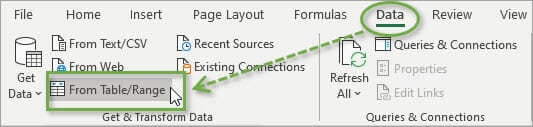
Go to the Power Query editor by clicking on From Table/Range on the Data or Power Query tab (depending on which version of Excel you are using).

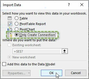
This brings up a preview of your data. To create a connection:

1. Click on the bottom half of the Close & Load split-button.
2. Select Close & Load To…
3. That brings up the Import Data window. From here, select Only Create Connection.
4. Click OK.

You can see the connection you've just created in the Queries & Connections pane. If ever you don't see the Queries & Connections pane, you can open it by selecting that button on the Data tab in the ribbon.

This process of creating connections must be repeated for every table that you want to append. Again, you only need to do this work one time for the initial setup. However, here are a few tips to speed up the process.

Use the Table Connections Macro

Since creating and connecting lots of tables can be time-consuming, I've created a macro that automates it. The macro loops through all tables in the workbook and create a connection only queries for any table that do not have queries yet.

Here is the post with the VBA macro to create connection-only queries.

The macros runs on the Active Workbook. You can add the macro to your Personal Macro Workbook and add a macro button to the Ribbon or Quick Access Toolbar to run it on any open workbook.

Close & Load Settings

If you'd rather not use a macro, you can also shorten the process by changing the setting of the Close & Load split-button. The default for the top half of that button will load the output table to a new sheet, but you can adjust the settings so that it only creates a connection instead. To change the setting:

1. Go to the File menu.
2. Select Options and Settings.
3. Choose Query Options.
4. That will bring up the Query Options window, where you can select Specify custom default load settings.
5. Deselect the Load to worksheet option.
6. Hit OK.

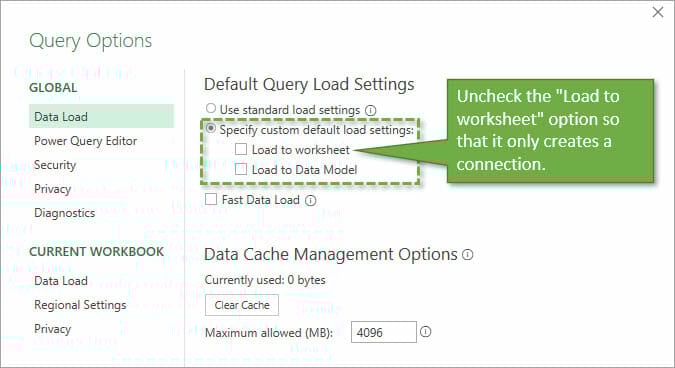
Just remember to change this setting back once you've finished connecting all of your tables.

2. Combining Connected Tables with Append

Once all of your tables are connected, it's a piece of cake to consolidate them:

1. Go to the Data tab.
2. Click on the Get Data button.
3. Select Combine Queries.
4. Choose Append.

This brings up the Append window, where we can select Three or more tables. This allows us to move any or all of the tables that we've connected from our Available tables (on the left) to the list of Tables to append (on the right).

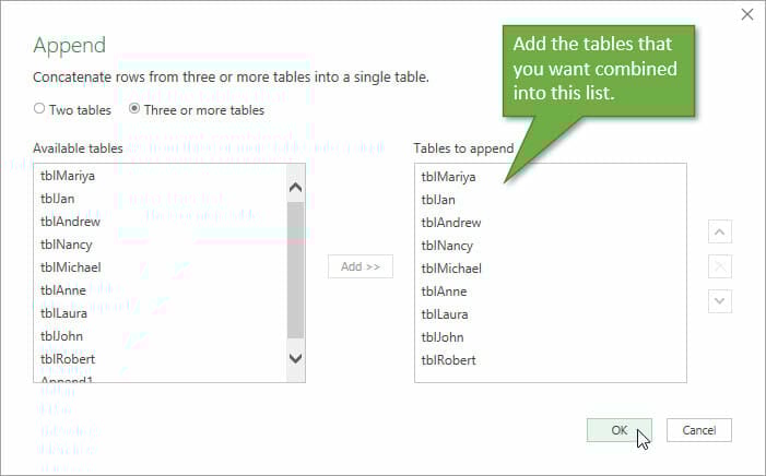
You can select all the Available tables by selecting the first table, holding Shift, then selecting the last table in the list. Then click the Add >> button to move them to the right side.

Once you hit OK, you will be taken back to the Power Query editor, where you can see a preview of the combined tables. You can make adjustments and transformations to the data before closing the editor and loading the data to a new worksheet.

Updating & Refreshing the Data

A great thing about Power Query is that you can refresh the output table any time there are changes made to any of the data sets. Just right-click anywhere on that output table and select Refresh.

This means we have fully automated this process. You do NOT have repeat the steps above every time your data changes or you get new rows in your tables.

Adding New Tables

If you ever want to add new tables to the query (or exlcude existing ones) you can reopen the Append window by:

1. Clicking on the output query in the Queries & Connections pane.
2. Opening the Query Settings pane if it's not already visible (View tab, then Query Settings).
3. Clicking on the little gear icon next to Source.

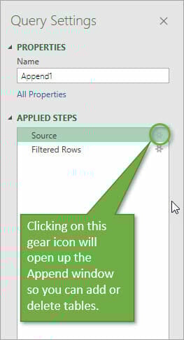
4. This opens the Append window, where you can add or delete tables.

Adding New Columns

One advantage of using Tables for this technique is that you do NOT have to make any changes to the query when new columns are added to the Tables. Power Query will automatically include the new columns in the query and output them in the appended query.

The new columns will still need to have the same column header name on each sheet. If any of the tables are missing columns, then Power Query will fill the rows for that table with blank (null) values in the append query and output table.

Other Power Query Posts

If you're just getting started with Power Query, check out my overview post here: Power Query Overview: An Introduction to Excel’s Most Powerful Data Tool.

Then get Power Query up and running with this tutorial: The Complete Guide to Installing Power Query.

Free Training Webinar on the Power Tools

Right now I'm running a free training webinar on all of the Power Tools in Excel. This includes Power Query, Power Pivot, Power BI, pivot tables, macros & VBA, and more.

It's called The Modern Excel Blueprint. During the webinar I explain what these tools are and how they can fit into your workflow.

You will also learn how to become the Excel Hero of your organization, that go-to gal or guy that everyone relies on for Excel help and fun projects.

The webinar is running at multiple days and times. Please click the link below to get registered and save your seat.

Click Here to Register for the Free Webinar

Conclusion

I hope this post was helpful in walking you through how to combine or consolidate sheets that have tables using Power Query. If you have any questions about it, please let me know in the comments. Thanks for following along!