This post will explain 7 keyboard shortcuts for the filter drop-down menus. This includes my new favorite shortcut, and it's one that I think you will really like!
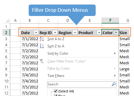
The Filter drop-down menus (formerly known as Auto Filters in Excel 2003) are an extremely useful tool for sorting and filtering your data. When the Filters are applied you will see small drop-down icon images in the header (top) row of your data range.
These menus can be accessed with keyboard shortcuts, which makes it really fast to apply filters and sorting to different columns in your table. So let's take a look at these shortcuts.
#1 – Turn Filters On or Off
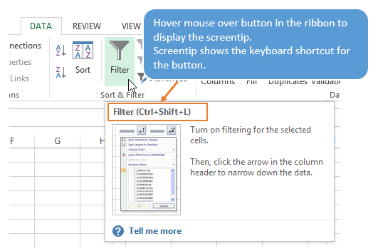
Ctrl+Shift+L is the keyboard shortcut to turn the filters on/off. You can see this shortcut by going to the Data tab on the Ribbon and hovering over the Filter button with the mouse. The screen tip will appear below the button and it displays the keyboard shortcut in the top line. This works with a lot of buttons in the ribbon and is a great way to learn keyboard shortcuts. See the image below.
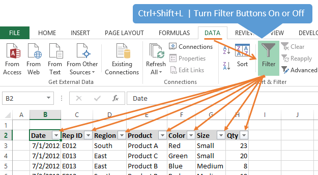
To apply the drop down filters you will first need to select a cell in your data range. If your data range contains any blank columns or rows then it is best to select the entire range of cells.
Once the data cell(s) are selected, press Ctrl+Shift+L to apply the filters. The drop down filter menus should appear in the header row of your data, as shown in the image below.
#2 Display the Filter Drop Down Menu
Alt+Down Arrow is the keyboard shortcut to open the drop down menu. To use this shortcut:
- Select a cell in the header row. The cell must contain the filter drop down icon.

- Press and hold the Alt key, then press the Down Arrow key on the keyboard to open the filter menu.
Once the drop down menu is open, there are a lot of keyboard shortcuts that apply to this menu. These shortcuts are explained next.
Bonus Tip: If you are using Excel Tables, and I highly recommend you do, you can press Shift+Alt+ Down Arrow from any cell inside the table to open the filter drop-down menu for that column.
This shortcut was introduced in Excel 2010 for Windows, and works in all newer versions as well.
#3 Underlined Letters & Arrow Keys
The underlined letters in the drop-down menu are the shortcut keys for each command. For example, pressing the letter “S” on the keyboard will Sort the column A to Z. You must first press Alt+Down Arrow to display the drop down menu. So here are the full keyboard shortcuts for the filter drop down menu:
- Alt+Down Arrow+S – Sort A to Z
- Alt+Down Arrow+O – Sort Z to A
- Alt+Down Arrow+T – Sort by Color sub menu
- Alt+Down Arrow+I – Filter by Color sub menu
- Alt+Down Arrow+F – Text or Date Filter sub menu

#4 Check/Uncheck Filter Items
The up and down arrow keys will move through the items in the drop down menu. You can press the Enter key to perform that action. This requires the drop down menu to be open by first pressing Alt+Down Arrow. See the image in #3 above for details.
Starting in Excel 2007, a list of unique items appears at the bottom of the filter drop down menu with check boxes next to each item. You can use the up/down arrow keys to select these items in the list. When an item is selected, pressing the space bar will check/uncheck the check box. Then press Enter to apply the filter.

#5 Search Box – My New FAVORITE
Starting in Excel 2010 a Search box was added to the filter drop-down menu. Excel 2011 for Mac users also get this feature.
This search box allows you to type a search and narrow down the results of the filter items in the list below it.

When the filter drop down menu is open, you can press the letter “E” on the keyboard to jump to the search box. This places the cursor in the search box and you can begin typing your search.
Alt+Down+Arrow+E is the shortcut to open the filter drop down menu and jump directly to the search box.
I just learned this shortcut and it is my new favorite because it makes it so fast to type and filter exactly what you are looking for in the list. Prior to learning this I was using the down arrow key to get to the search box. This required me to press the down arrow key 7 times to get to the search box. Now I can do the same thing in one step by pressing the letter “E”. What a time saver!
Bonus – Jump to the Checkbox List
If you want to jump down to the checkbox list below the Search box, you can just press Tab after Alt+Down Arrow, E.
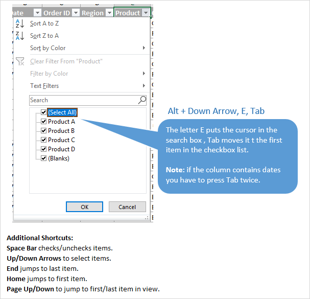
So the full keyboard shortcut is: Alt+Down Arrow, E, Tab (or Down Arrow)
You can use either the Down Arrow or Tab keys. Down Arrow will probably be easier since you just pressed Down Arrow to open the filter menu.
However, if the column contains dates then you need to press Tab twice. There is an additional drop-down menu to search by Year, Month, Date. Down Arrow opens that menu and selects each item.
Therefore, it's probably best to get used to using Tab to get there since it works in all situations.
Once you press the shortcut, focus will be set to the (Select All) checkbox in the list box. You can then use the following shortcuts to navigate and select the checkboxes.
- Space Bar checks/unchecks items.
- Up/Down Arrows to select items.
- End jumps to last item.
- Home jumps to first item.
- Page Up/Down to jump to first/last item in view.
#6 Clear Filters in Column
Alt+Down Arrow+C will clear the filters in the selected column. Again, this is a combination of the Alt+Down Arrow to open the filter menu, then the letter “C” to clear the filter.

This would be the same as pressing the (Select All) checkbox in the item list. The next shortcut will explain how to clear all the filters in all columns.
#7 Clear All Filters
Alt+A+C is the keyboard shortcut to clear all the filters in the current filtered range. This means that all the filters in all the columns will be cleared, and all rows of your data will be displayed.
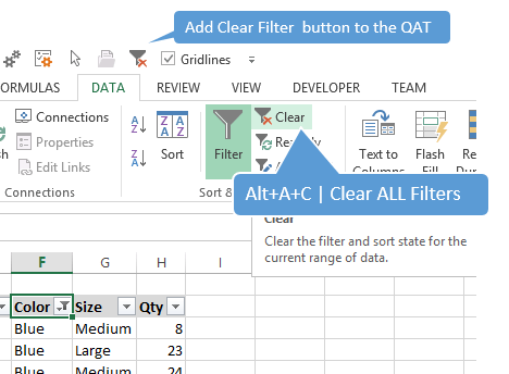
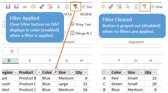
I add the Clear Filter button to the Quick Access Toolbar (QAT) and would highly recommend that you do this. It serves two purposes that are very helpful.
- You can quickly press the button in the QAT to clear the filters. If you are a mouse user this means you don't have to navigate to the Data menu to access the button. You can also use keyboard shortcuts to press the buttons in the QAT. See my articles on how to setup the Quick Access Toolbar and how to use the QAT's keyboard shortcuts for instructions on this.
_ - Use the button to visually see if any filters are applied. This is the most important benefit to me. If any filters are applied to the filter range, then the Clear Filter button in the QAT will show color (enabled). If no filters are applied then the button is grayed out (disabled). See the image below for details.
_
Debra Dalgleish has a great post and video with a few additional tips to Clear Excel Fitlers with a Single Click over at the Contextures blog.
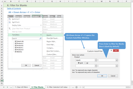
#8 Filter for Blank or Non-blank Cells or Rows
Alt+Down Arrow+F+E+Enter will filter for blanks cells in the column.
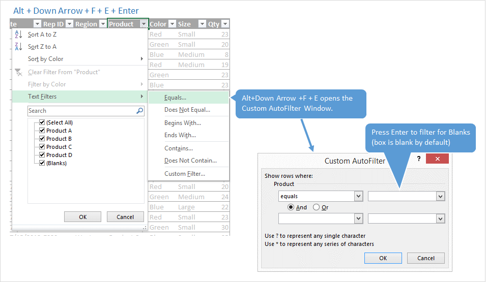
The F,E combo opens the Custom AutoFilter menu where you can type a search term. The box is blank by default. So if you just hit Enter when the Custom AutoFilter menu opens, the column will be filtered for blanks.
This is another one of my new favorites! It's much faster than unchecking the Select All box, then scrolling to the bottom of the item list.
You can also filter for Non-blanks using the shortcut Alt+Down Arrow+F+N+Enter. This opens the Custom AutoFilter menu and sets the comparison operator to does not equal. The criteria is blank by default, so this applies a filter for non-blank cells. Thanks to Nilesh for leaving a comment and inspiring this one!
Bonus Tip
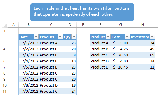
Typically you can only have one range filtered on a sheet at a time. This means that if you have more than one range of data on a sheet, you can not apply the Filters menus to both ranges.
If you use the new Excel Tables feature (introduced in Excel 2007 and available for 2011 for Mac) then you can apply Filters to each table in the same worksheet.
Checkout my video tutorial on Tables to learn more about all the great time saving benefits they have to offer.
Want More? – Download the Workbook
I hope you've learned some new tricks that will save you time when working with Filters. In my opinion, the keyboard shortcuts are the fastest way to work with these menus. I encourage you to practice these techniques, and also share them with a friend that might benefit.
I have also created a free workbook that contains over 25 keyboard shortcuts for the Filter Menus. The workbook is organized by topic and contains images that will help you learn the shortcuts. It also includes a data table where you can practice the shortcuts.
Please fill out the form below to download the file immediately.
You will also have the option to subscribe to my free email newsletter to stay updated with new articles and videos that will help you learn Excel. After confirming your subscription you will be able to download my “10 Excel Pro Tips” eBook. It's all free!
Challenge Question
What does the following keyboard shortcut sequence do? The selected cell must be in the header of a filtered range.
Alt+Down Arrow+E, Down Arrow, Space Bar, Shift+End, Space Bar, Enter
Please leave a comment below with your answer. Thanks!


Hi Jon,
Thanks for the excellent article. Your tips are now saving me a lot of time!
A question though-
Is there a shortcut to select multiple values in the drop down filter. I normally work with large sets of data, and the filters can range from 50 to 100. for eg., my data may have options from 1990 to 2050. But i am required to select only from 1990 to 2000.
What i doing currently is to move the down arrow and hit spacebar for each of the individual values i want.
Hi Anurag,
Great question! I usually do the spacebar/down arrow technique as well. For the example you gave you could use a number filter for numbers between. The keyboard shortcut is Alt+Down Arrow, F, W. That will open the custom auto filter window and you would type 1990, tab 3 times, type 2000, hit enter. It would be faster if you had a large range to select. I hope that helps. Thanks!
Hi Jon,
sorry buddy its not working,
could you share example excel file for this
ThanQ
It is Alt + DownArrow , F and then E.
Thanks alot for your huge experience
Problem:
I have done excel sheet with huge data entered and used filters to enter data easely also used CTR + ENTER for quick entering data
When I nearly finished my sheet found data entered are not the same I typed . Like eneterd data inserted in hidden rows and cells ?
How come ? Filters deals with visible cells only not hidden where is the problem?!!
Hi Sherif,
That sounds frustrating. I’m not exactly sure what the problem might be. Whenever I am working with a filtered range and have a range selected, I always use the Select Visible Cells keyboard shortcut (Alt+;) to select the visible cells first. Even though the range is filtered I have also experienced issues with hidden rows being modified.
To be safe I always select visible cells first. Here is an article and video that discusses the visible cells shortcut in more detail. I hope that helps. Let me know if you have any questions. Thanks!
Great !!!
Great! thank you
Hi Jon,
Thanks for good information about filter shortcut key.
And your thinking must great .
Thanks a lot Jon!
Ranjit, use the FOFO method to do that:)
Pls mention Alt+A+T instead of Alt+A+C is the keyboard shortcut
Hi Rajiv,
Thanks for the suggestion. Alt,A,T is the keyboard shortcut to turn the filters on/off in the English version of Excel. You can also use Ctrl+Shift+L to turn the filters on/off. Alt,A,C is the keyboard shortcut to clear filters. I hope that helps. Thanks!
Very useful shortcut keys. Thank you EXCEL CAMPUS. 🙂
Awesome! Thanks Khaleel! 🙂
hijon,
I have numerous items in the list box , instead of pressing down arrow in the keyboard how can I go to the end of the list box and select the particular item.
Hi Abi,
The End key is the keyboard shortcut that will select the last item in the filter drop-down list box. You just have to have an item selected in the list first. Thanks!
Hi,
sorry I have a question related to the filter but not necessarily on this topic.
I use a lot the filter when preparing charts (scatter mainly) comparing data with different characteristics. The problem that I have once I have filtered the data is that I have to select the each one separate data for the chart, because if I select the entire column the chart will display the hidden data too.
Is there any way to avoid this tedious work?
Thank you
Hi Giacomo,
I’m not sure I understand your question. The data should not display in the chart if you have the source data filtered.
Grate! thanks a lot my friend these are very helpful thanks again
Thanks Rahat!
Hi Jon,
Is there any shortcut key for choosing items inside the ‘List’ formed by Data validation. I use Alt+Down arrow to open the List items, but after that I am bound to use mouse to choose/select the data inside the list..It should be searched by alphabetically as in Filter. Pls suggest me.
Hi Pradipta,
Unfortunately, validation does not have these features built into it. It would be nice though… 🙂
Jon,
I stumbled across your article and thought you might be able to help. Is there a way to display which filters have been selected? If you hover over a filter drop down button, it will actually display which filters have been applied. Unfortunately, I can’t seem to find where/how this information is stored so that I can display it in another cell.
I have a spreadsheet with several thousand lines. I have a column with about 12 distinct entries. My goal is to create a cell on a summary page that tells you which of the 12 filters, or combination there of, that are currently selected.
I’m thinking there might be a brute force way to do it where I use a bunch of drop downs that match the filter options, then feed that into a custom filter somehow but that seems extraordinarily labor intensive for something that Excel already has calculated somewhere.
Thank you,
Joe
Hi Joe,
Great question! The current filter criteria can be accessed by a macro (VBA). I am actually working on an add-in that does exactly this, and allows you to see and quickly navigate to the filtered columns. It also displays the filter criteria for each column. I’m hoping the add-in will be out in the next month.
In VBA you can use the AutoFilter object and properties to find the criteria for each filtered column in a range or Table. I will have more articles on this in the future as well. Please let me know if you have any questions. Thanks!
Hi Jon,
Your article is really helpful. I am using data filters in excel and often I encounter a + sign in the months column. I have to click on that + sign to expand the dates for that specific month. Is there a shortcut key to expand the + sign in data filter and see the dates for that month.
Hi Saravan,
Great question! The Right Arrow Key should expand the grouped date items in the filter drop-down menu. When the item is selected in the list, press the right arrow key. That will expand the group. You can then press the down arrow key to select items below, and further expand months, days, times, with the right arrow key. I hope that helps. Thanks!
The left arrow key will collapse the group as well.
Is the answer to the challenge question – filter by blank cells?
Hi Rob,
Yes, that is the answer. The column needs to contain blank cells for it to work. I should have prefaced that.
An easier way to filter for blanks is Alt+Down Arrow, F, E, Enter. That will set the Text Filter equal to blank.
Thanks for answering the question. 🙂
Awesome shortcuts, Jon! I also agree that the one to get to the search box is especially good. I have just been tabbing a bunch of times to get to it. 🙁
I’m struggling a little with the steps to get the answer to the challenge question. I don’t see why one of the steps is to do Shift + End. I seem to get the same result without holding Shift when I press End. Is there a reason to do Shift + End at this step?
Hi jon,
Can we paste into visible cells directly? or using any shortcut keys or method? Thank you. 🙂
Hi Pooja,
Not directly with Excel, however, my Paste Buddy add-in has a feature called Paste Visible that does this. Here is a video with more info on the problem and solution. I hope that helps.
can we print the drop down list after applying the filter
Hi Chandra,
I don’t believe there is a way to print the filter criteria without using VBA. I will post an article that explains how to get the filter criteria with VBA. Thanks
This might not be precisely what you want but if you open the filter with a keyboard shortcut but keep the alt key selected. Then press the printscreen key and that puts the drop down list in your clipboard. Then go to where you want the drop down list and press cltr + v.
btw – very useful tips. Thanks!
Hi Mark,
Wow, never knew that one. I’m only able to get a screenshot of the drop-down menu though. Does it actually put the values in the clipboard and paste them to cells for you?
Great article! This Alt+Down+E is my new favorite as well… I needed this so bad!
Awesome! Thanks Paulo! 🙂
Hi Jon.
Is there a way to expand the table while filtered? i hate when i want to add something for that specific person, i have to unfiltered everything in order for it to work. Please help thanks.
Hi Chau,
If you are using an Excel Table then it should automatically expand when filters are applied. Checkout this video on Excel Tables if you are not using them yet. They are an awesome tool!
It’s really helpful… Thanks Jayavelu Sampangi
Thank You Jon !!
In case of a non-blank range, the last of the filterable options are chosen.
Hi Jon,
Thank you for this excellent article.
Regards,
Hilary
Thanks Hilary! 🙂
God stuff. The only thing that does not make sense to me is:
* Select a cell in the header row
* Press and hold the Alt key
* press the Down Arrow key on the keyboard to open the filter menu.
This is much longer than clicking on the filter icon directly to open the filter menu. I cannot see how you can recommend replacing 1 step by 3 steps when you are talking about productivity improvement, which is what keyboard shortcuts are about.
1st word should be “Good” instead of “God”. My apologies.
Klaas, if you are in the table in spreadsheet, press ctrl+above arrow to reach at the header row. Then click on Alt+down arrow… bingo!…. If you want to filter different heads a number of times, this command saves a lot of time.
Jon, excellent article!
Thanks
Thanks Ghani! That is a great suggestion. As I mentioned to Klaas, if you are in an Excel Table then you can press Shift+Alt+Down Arrow to open the filter drop-down menu for the column of the selected cell. You do not have to select the header cell first.
I will update the article to include this.
Hey Klaas,
Sorry, I missed your comment here. As Ghani mentioned, you can jump to the header cell by pressing Ctrl+Up Arrow if you have a cell selected in the column you want to open the filter menu for.
If your data is in an Excel Table, then you can press Shift+Alt+Down Arrow in any cell in the table to open the filter drop-down menu for that column.
The choice between using the keyboard or mouse will depend on where the selected cell is in comparison to the filter drop-down menu you want to open. The mouse can be faster in some cases.
In my opinion it’s great to know the keyboard shortcuts, as they can save you a lot of time in the right situations. I am not stating that one is faster than the other in all occasions. Using keyboard versus mouse shortcuts is highly dependent on what the user feels comfortable with. Not all hands and fingers were created equal… 🙂
I hope that helps. Thanks again!
Hi Jon,
As you know, mac shortcuts are often different than windows’..
The one I cannot figure out is “#4 Check/Uncheck Filter Items” in Excel 2016 for Mac
Do you have any idea (spacebar will not do it)?
Thank you in advance for your attention.
R.I
Great question R.I. Unfortunately I don’t know that there is one. I could not figure it out either. I would recommend posting this issue on Excel Uservoice for Mac. The Excel product team uses this platform to enhance the product. Thanks!
Merci Jon, J’adore vos articles. J’ai appris encore un fois une nouvelle astuce.
Amicalement, Mariem
Thank you Merimar! 🙂
Thanks a lot.
#8 : try pressing “FF” instead of “FE”, after you press ALT + DownArrow … even faster!
You can also just press Enter twice after pressing ALT + Down Arrow, F.
these shortcuts are very use full for me, thanks a lot, can you tell me how to find duplicate entry one sheet to another sheet?
Hi Aman,
You can use the COUNTIF Function to find duplicates, or you can use a pivot table to compare lists. I hope that helps.
Thanks these are very useful again thanks for your support.
Hi Jon,
Do you know of a way to increase the height of the filter dropdown?
The tiny filter dropdown only shows 8 or 10 values. I have to constantly grab the bottom right corner and stretch the list down to see a reasonable number of items.
Is it possible to:
1) Use shortcut keys to double or triple the height of the filter window?
2) Change that default so it always shows 20, 30, 40 items by default?
Thanks, Jon!
Hi Dave,
Unfortunately, it’s not possible to set the default size (height or width) of the filter drop-down menu. I have asked the Excel team about this.
You can also turn the filter on/off for blank cells by typing “blank” into the search bar! Saved me a number of times when my data set is too large for the blank option to be displayed. Little faster than some of the other options I think.
Great suggestion! Thanks Trish! 🙂
Do you know the shortcut to “reapply filter” when a new criteria applied?
Alt,A,Y is the keyboard shortcut to the Reapply button on the Data tab of the ribbon.
Ctrl+Alt+L – as shown on the tool-tip option.!
Jon,
I would like to set up my spreadsheet to assign certain keys to a function. Specifically I have a drop down boxes and when that cell is highlighted I want to press a single key to perform a function. For instance when a box is highlighted and the options are yes and no, I would like to press b for yes and n for no. Any tips on how to set this up?
Hi Tony,
You could use a macro for this, or you create a separate column with an IF formula.
I don’t have any articles on the macro, but I will add it to the list for the future.
Thanks!
Those are some nice bonuses in the downloadable file!
Anyone who hasn’t opened up the file and seen the command to “Filter by Selected Cell’s Value” is really missing out. This is another command that I like having on the QAT, since it is not on the ribbon, and I didn’t know it was in the right-click menu. You can add it to the QAT by looking at the “Commands Not in the Ribbon” dropdown, and it is called AutoFilter.
Thanks John! That is a great suggestion! 🙂
thank you very much, it’s so useful and helpful
Very very very very useful and awesomely explained. worth a read and use….
Thanks Sir.
Hi there,
Thanxs for the info but do you have any idea that how to apply filter when u have pictures in your excel file because when i apply filter all my pics collage and it creates a mess
Good and very useful information.
Kishan Kapoor
Hi Jon,
Thanks for the shortcut key. It’s very good and very useful.
Thank-Q
Hi Jon,
This is of great help, please keep on posting such articles, really useful, it would be nice if you can do same for ppt as well.
Thanks
Hi Jon,
Thank you for this excellent article.
Regards,
Anurag
Hi Jon,
whether converting excel range to excel table increases the file size ?
Thanks for the excellent article. Your tips are now saving me a lot of time!
Hi,
In excel sheet 1000 Columns Value available in one Sheet. Now we apply Filter Condition in 1000 Columns If i See the One Column Value i apply the filter i see the Values in each column and One Small box also Appear and We Click the Box Which Item Value required and We will See the Value. Now how to go directly last see Value inbox ? So kindly help this Question and rectify immedaitly
Thanks for your information.
I want to know 2 function shortcut key of wps spread sheet.
1. How to appear and remove shortcut key of auto filter (i tried ctrl+shift+L its not working)
2. How to select shortcut key of column select
Alt+Down Arrow+E, Down Arrow, Space Bar, Shift+End, Space Bar, Enter
It is used to tick the Blank cells in the data range.
excellent, clear, simple and efficient… alt+down,alt+e my new favorite
Alt + Down Arrow. It’s the best absolutely!
HiJon,
i have made hide the column, how i make unhide with out selection the cells
Hi Jon,
First off, thank you for giving the public access to these tools. You’re saving everyone a lot of time. My favourite one so far is the drop-down list search which I now use multiple times a day. I am however having an issue every time I close all excel files. Once I re-open them, the XL Campus tab disappears regardless of the plug-in still being selected in Options. The only solution I’ve found was to remove the plug-in and add it once again.
Have you come across this issue before? If not, then I’ll know it’s something to do with my computer
Thanks!