You can write a lookup formula that returns multiple values using tools like VLOOKUP or XLOOKUP, but the FILTER function in Excel is a faster and easier option.
Video Tutorial
Watch on YouTube & Subscribe to our Channel
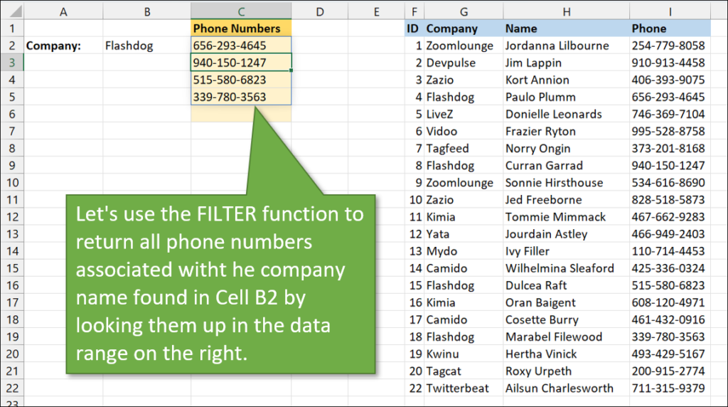
For example, I want to look for a specific company name in a range of data and return any phone numbers that are associated with that name.
The FILTER Function
Let's walk through the steps to write this function.
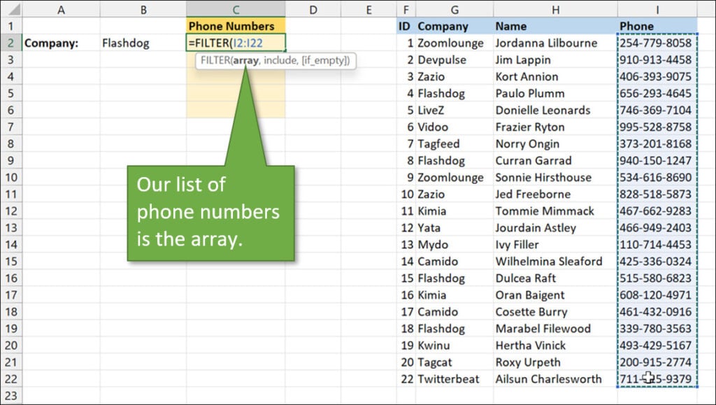
1. Start by typing the equal sign = and the word FILTER, then hit tab.
2. There are three arguments in this formula. The first is array, which is the range of cells that that we want to return values from. In this case, the phone numbers.
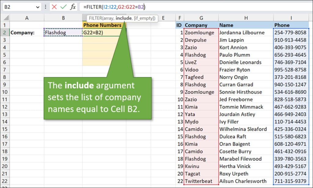
3. Next is the include argument, which is our filter criteria. For our example, we will take the list of companies and set it equal to cell B2.
4. Then, for the [if empty] argument, you can type whatever you want in quotation marks, such as “Not found.”
![Filter function
[if empty] argument](https://www.excelcampus.com/wp-content/uploads/2023/02/image-1-3-1024x620.jpg)
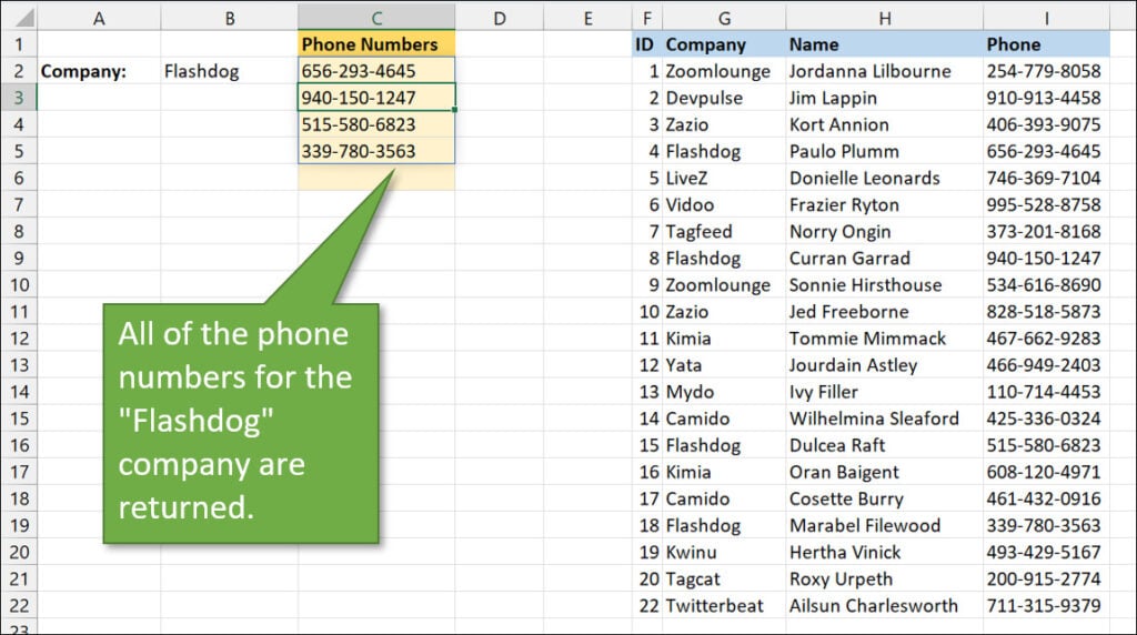
Finally, with all of our arguments written, we can hit Enter, and you will see that all of the phone numbers associated with the specified company spill into the cells below our formula.
Conclusion
Hope this quick overview of the FILTER function helps you to give it a try in one of your spreadsheets. Leave a comment if you have questions or feedback!


Excellent explanation! Thank you!
Is it possible to use multiple criteria using the AND function?
Excellent, I’m hoping to use this in place of the the vlookup formula. This Filter option seems like a much easier formula than vlookup. Also vlookup needs to be sorted and cannot find multiple occurrences. I’ll use the filter option in the future.
When using the filter function, if the argument has more than one, the results will give me a “Spill!” error. What is your recommendation for this issue? (for example, in your learning tips, if Zazio is listed more than once, then I get the Spill! error).
If you have anything in the cells below the SPILL error, they have to be cleared. For example using the above, if you have something typed in C4, then you will get a SPILL error because all the data can’t “SPILL” down the column. If you clear C4, then the SPILL error should be resolved.