

Download the Excel Files
Complete the form below to instantly access the Excel files and Excel Formula Prompting Guide.
Video Tutorial
Microsoft just dropped one of the most significant Excel updates in years. Lists in cells let you store multiple values inside a single cell as a true structured list, and the rest of the update builds from there. You get smarter filtering, four brand-new functions, collapsible arrays, and even nested arrays. This post walks through each piece so you can start using these features as soon as they hit your version of Excel.
What Are Lists in Cells?
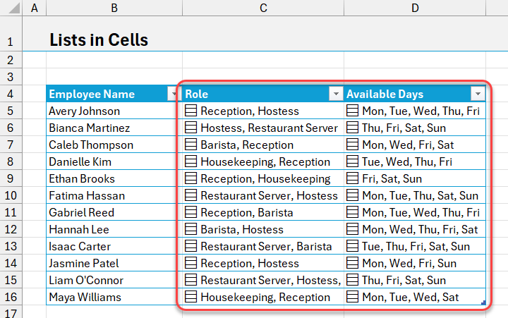
A list in a cell is a comma-separated set of values stored as a structured object, not just plain text. You can spot them by the small card icon on the left side of the cell. Click that icon to preview all the values in the list.
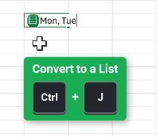
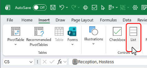
Creating a list is simple. Type a comma-separated value in a cell, then press Ctrl+J. That shortcut instantly converts the text into a list in a cell. You can also select an entire range of existing comma-separated values and press Ctrl+J to convert them all at once. There is also a button on the Insert tab if you prefer the ribbon.
Once a column contains lists, Excel gets smart about new entries. If you type a comma-separated value below existing list cells and press Enter, Excel recognizes the pattern and converts it automatically without needing Ctrl+J.
Filtering by List Items
Once you have list-in-cell columns, the Filter drop-down changes. Instead of showing the full comma-separated string, it breaks each list into its individual values. So if a cell contains Mon, Tue, Wed, Thu, Fri, the filter drop-down shows five separate checkboxes.
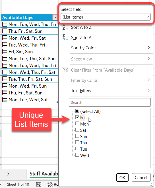
The column is filtered for items doing a contains type filter for the items within the lists in cells. So any list that contains “Fri” will be displayed in the results. This is easier and more accurate than doing a Contains type filter for cells that might contain a comma separated list but aren't converted to a list.
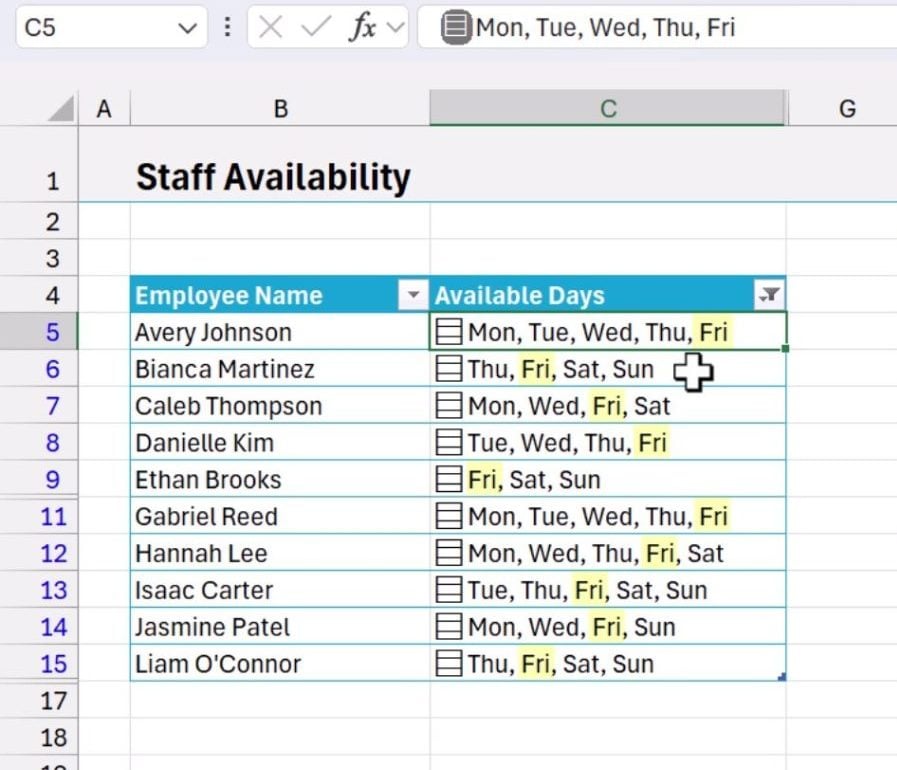
A new ‘Select field' drop-down appears at the top of the filter menu. You can switch between ‘List Items' (the individual values) and ‘Display value' (the full comma-separated text). List Items is the default for list-in-cell columns. You can stack filters across multiple columns too, which makes it easy to find, say, baristas who are available on Saturday.
The HAS Function: Check If a List Contains a Value
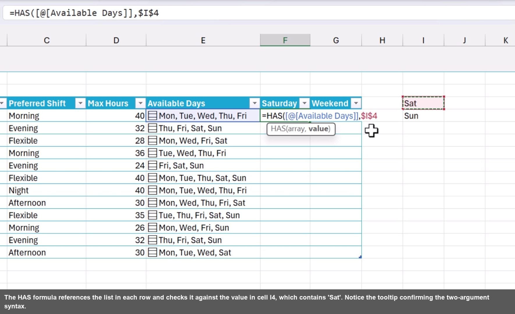
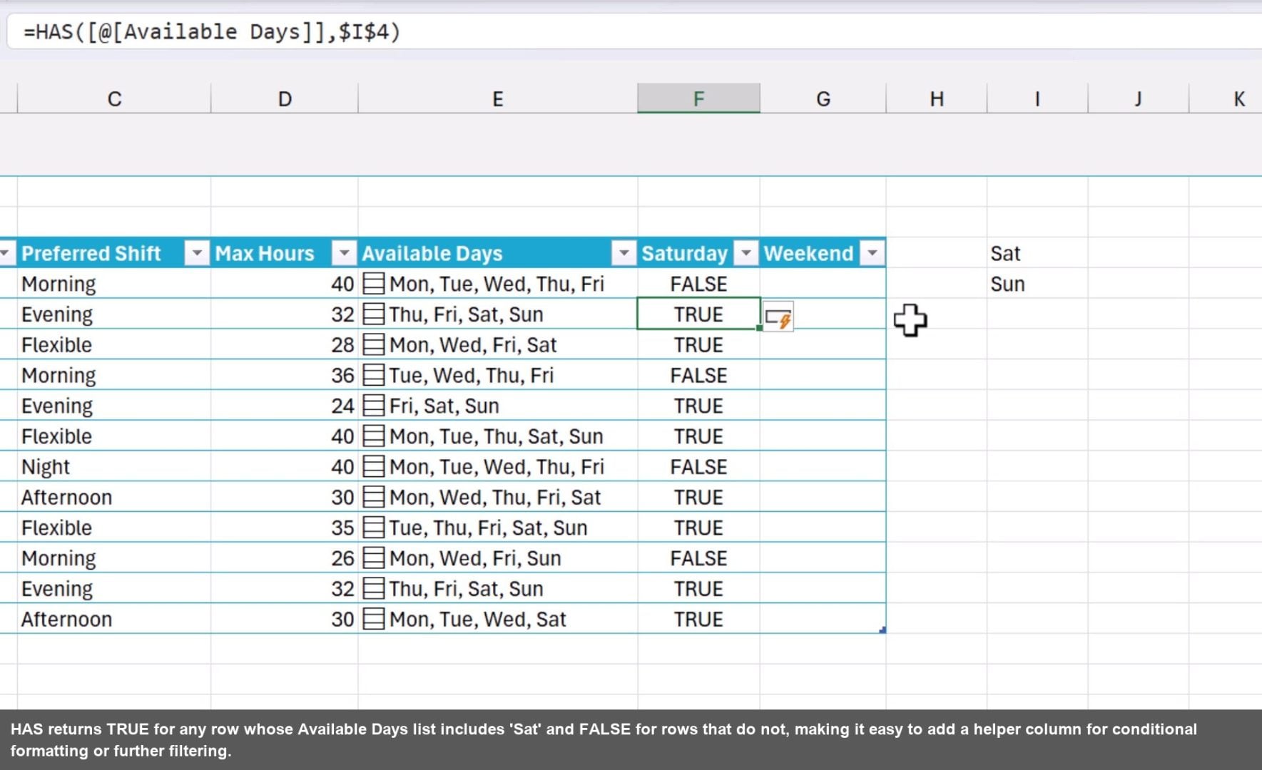
Formulas get a major upgrade here too. The HAS function lets you test whether a list in a cell contains a specific value, returning TRUE or FALSE. This is perfect for building helper columns that drive conditional formatting, FILTER formulas, or dashboard logic.
Here's a quick look at the HAS function. It checks whether a list or array contains a specific value and returns TRUE or FALSE. The function arguments are:
- array: the list or range to search through, typically a list-in-cell column
- value: the single value to look for within the array
=HAS([@[Available Days]],$I$4)
HASALL and HASANY: Check for Multiple Values at Once
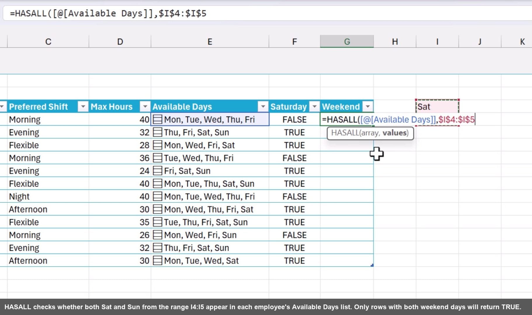
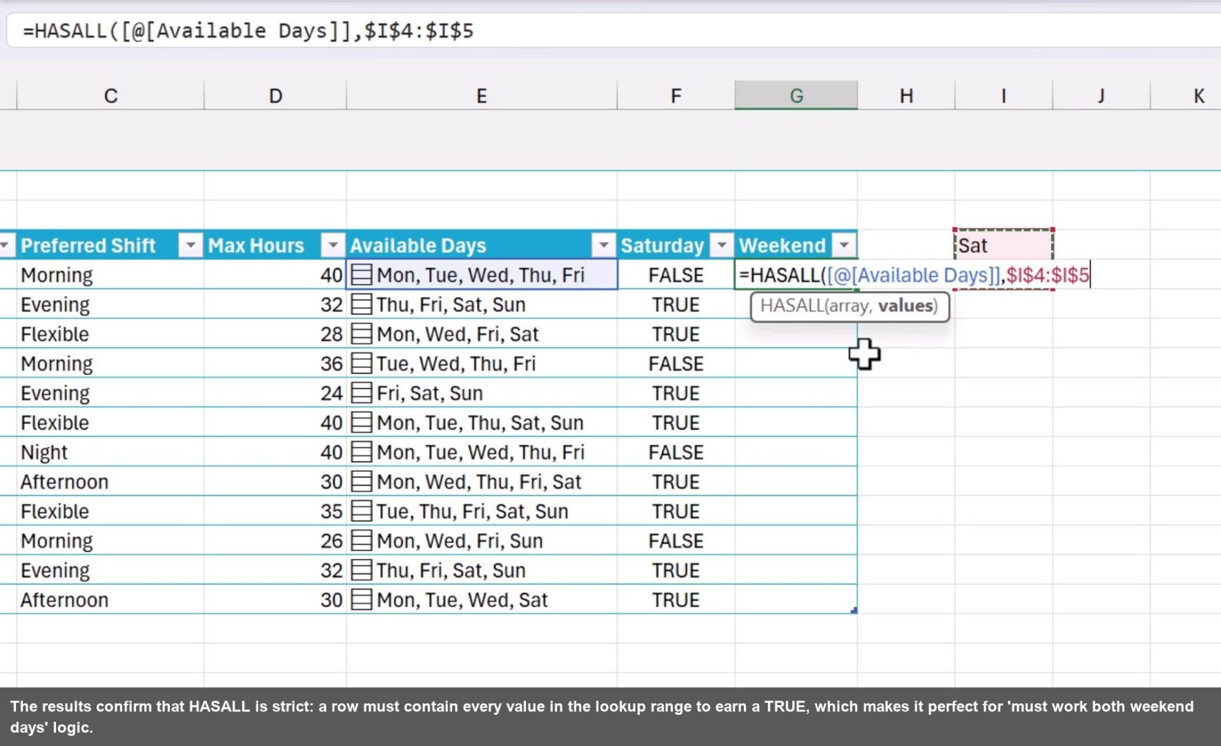
When you need to test for more than one value, two additional functions handle the logic. HASALL returns TRUE only when every value in your reference list appears in the cell. HASANY returns TRUE when at least one value matches.
A great trick here: you can store your lookup values as a list in a cell, then reference that single cell in your formula. Instead of pointing to a range like I4:I5, you put Sat and Sun into one list cell, press Ctrl+J, and reference that cell. Cleaner spreadsheet, same result.
Before diving in, a quick look at HASALL. It returns TRUE when a list or array contains all of the specified values. The function arguments are:
- array: the list or range to search through
- values: a range, list, or array of values that must all be present in array
=HASALL([@[Available Days]],$I$4:$I$5)
In case we're new to HASANY, it returns TRUE when a list or array contains at least one of the specified values. The function arguments are:
- array: the list or range to search through
- values: a range, list, or array of values where any one match returns TRUE
=HASANY([@[Available Days]],$I$4:$I$5)
Collapsing Lists Inside an Excel Table
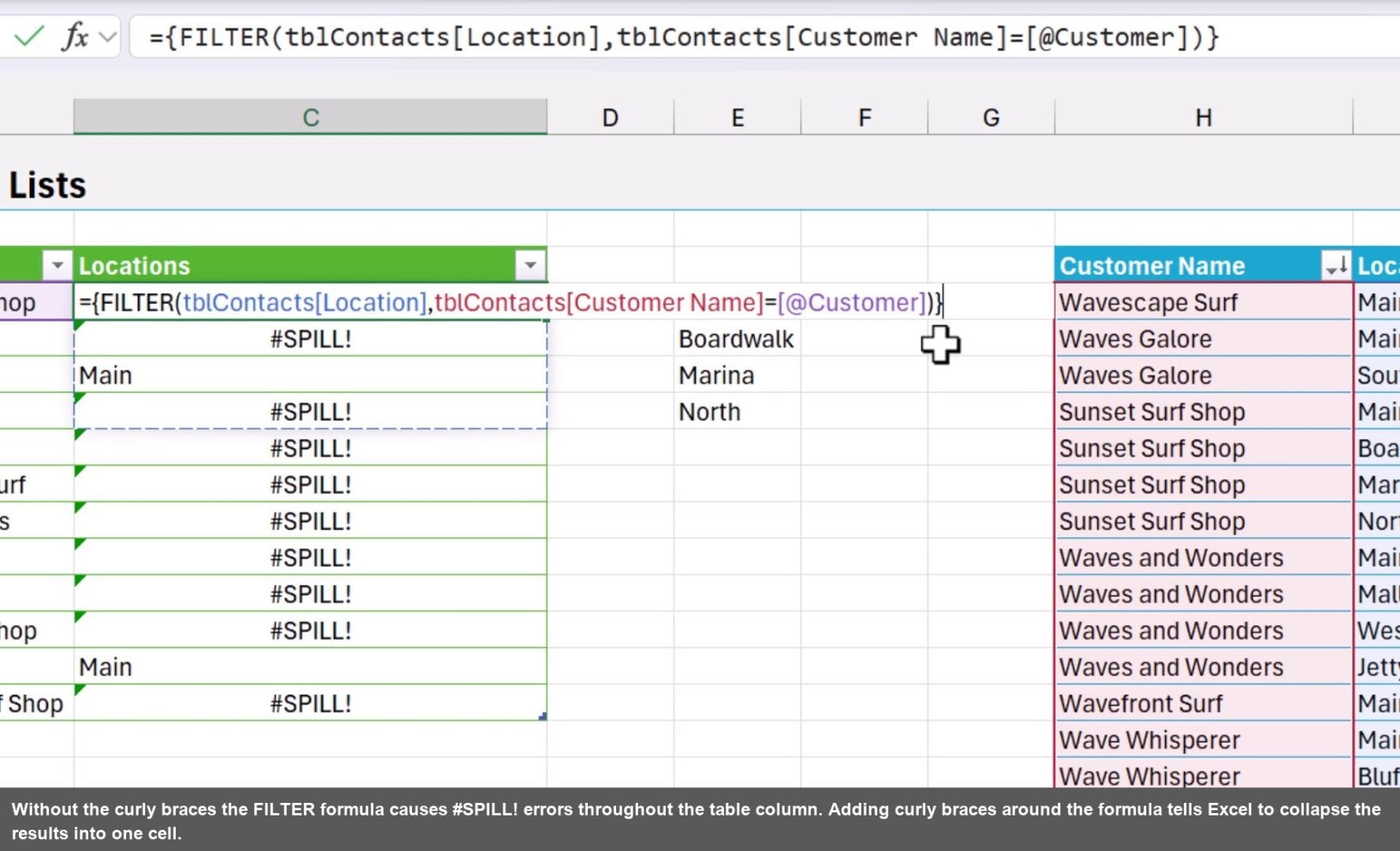
One of the most practical upgrades here is the ability to collapse a spilling formula into a list in a cell. Normally when you use FILTER inside an Excel Table, you get a cascade of #SPILL! errors because the formula tries to spill into rows below it that are occupied.
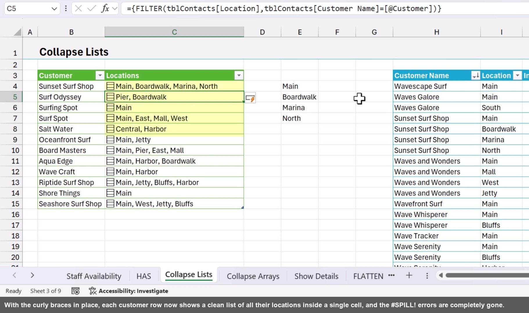
The fix is simple: wrap the entire formula in curly braces. Put an opening curly brace right after the equals sign, and a closing curly brace at the very end. That tells Excel to collapse the results into a single list in a cell instead of spilling down. No more TEXTJOIN workarounds.
A brief word on the FILTER function. It returns a subset of a range or array based on a condition you define. The function arguments are:
- array: the range or array to return rows from
- include: a boolean array the same height as array that tells FILTER which rows to keep
- if_empty: value returned when no rows match (optional)
={FILTER(tblContacts[Location],tblContacts[Customer Name]=[@Customer])}
Arrays in Cells: Store 2D Data in a Single Cell
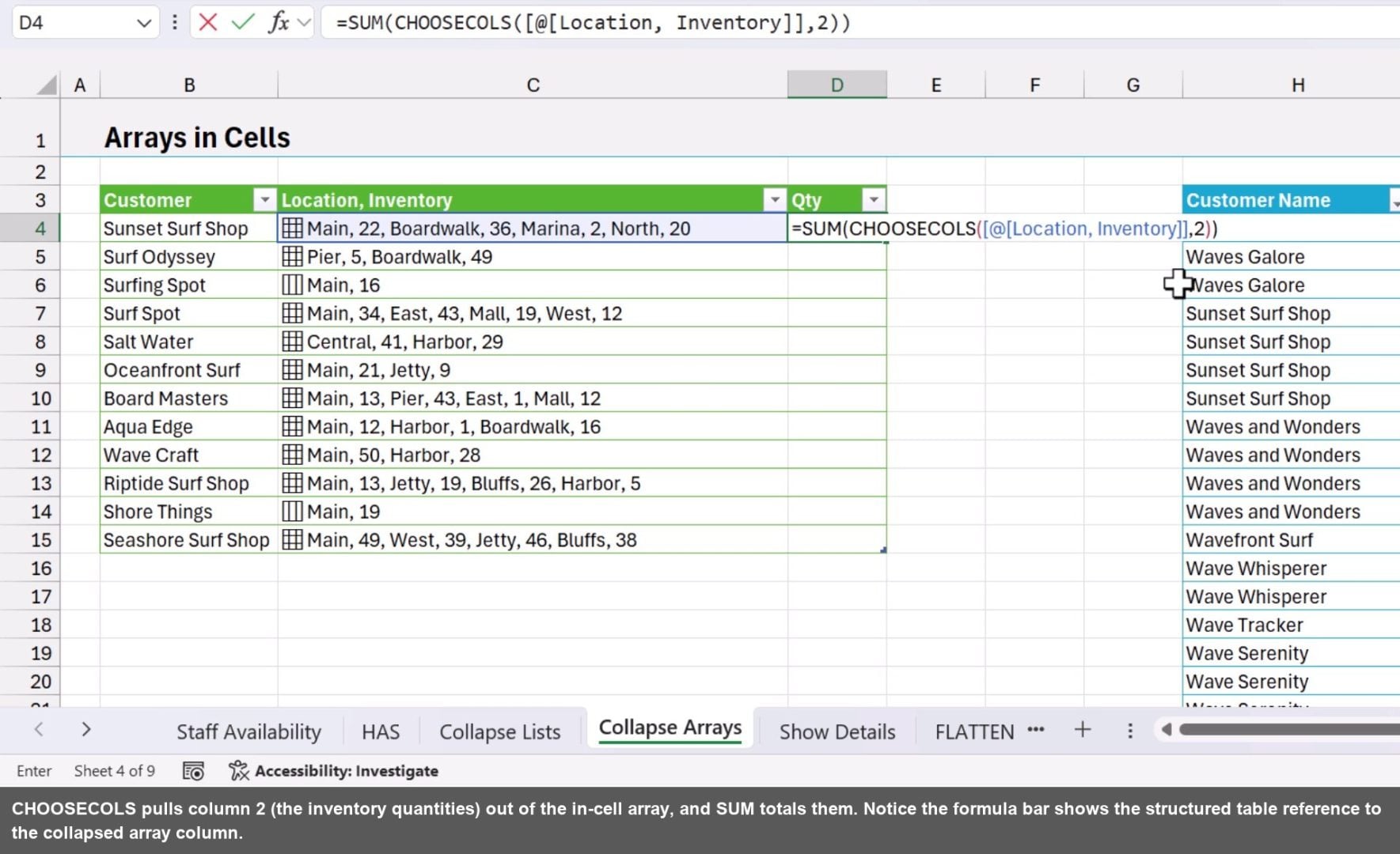
The curly brace trick also works when your FILTER formula returns multiple columns. The result is an array in a cell, a two-dimensional structure stored in a single table cell. The card icon looks slightly different from a standard list, and clicking it shows both rows and columns in the preview.
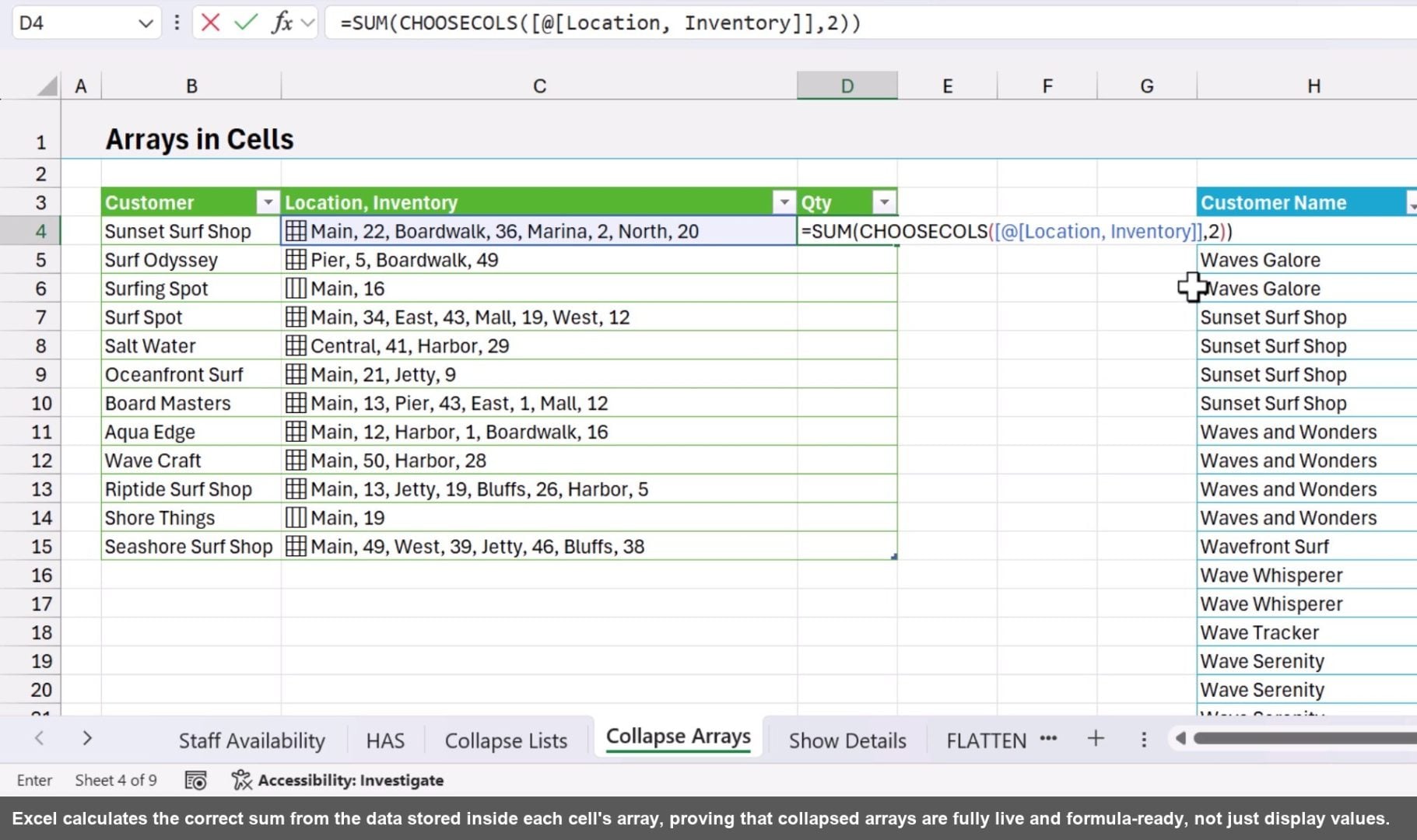
The remarkable part: you can run any Excel function directly on that in-cell array. Want to sum just the inventory column from the collapsed array? Use CHOOSECOLS to pull that column, then wrap it in SUM.
A quick look at CHOOSECOLS before we use it. It returns specific columns from an array by column number. The function arguments are:
- array: the range or array to extract columns from
- col_num1: the column number to return; add more col_num arguments to return additional columns (optional)
=SUM(CHOOSECOLS([@[Location, Inventory]],2))
Nested Arrays and the FLATTEN Function
Things get genuinely powerful when arrays contain arrays. Imagine an orders table where each row holds a collapsed FILTER result for order details, and those details themselves contain size lists. That's a nested array, and you can drill into it level by level using the card preview.
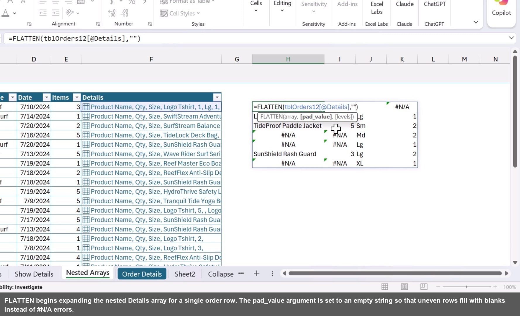
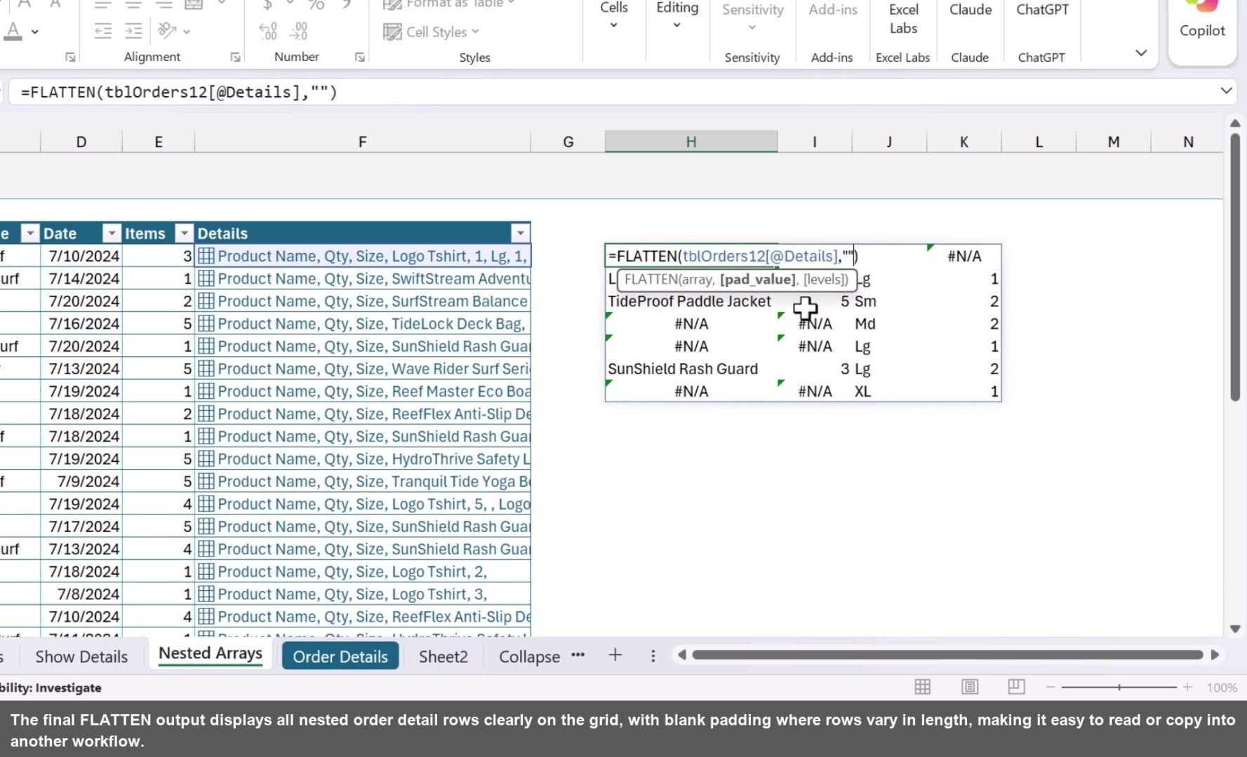
When you need to get that nested data back onto the grid, use FLATTEN. It expands nested arrays into a standard spilled range. The pad_value argument lets you replace structural gaps with blanks or any value you choose, keeping the output clean.
Here's a quick refresher on the FLATTEN function. It expands nested arrays or lists in cells out onto the grid as a spilled range. The function arguments are:
- array: the cell or range containing the nested array to expand
- pad_value: a value used to fill structural gaps when arrays at different levels have different widths (optional)
- levels: how many levels of nesting to flatten; defaults to all levels (optional)
=FLATTEN(tblOrders12[@Details],"")
Summary
The lists in cells update is one of the biggest structural changes to Excel in a long time. You can now store multiple values in a single cell as a real list, filter by individual items inside those lists, and use HAS, HASALL, and HASANY to build formulas that test for one or many values.
Wrap a FILTER formula in curly braces to collapse it into a list cell and eliminate spill errors inside tables. Push further with 2D arrays in cells, calculated using any Excel function via CHOOSECOLS or similar. And when nested arrays need to come back to the grid, FLATTEN handles it cleanly.
These features are currently rolling out to users on the Microsoft 365 beta channel, so keep an eye on your version for when they arrive.




Excellent
Its amazing to learn new excel feature, Thank you for sharing
Wonderfull