2-Way XLOOKUP in Excel: Beginner to Advanced

Bottom Line: Master the 2-way XLOOKUP to streamline your Excel skills—covering everything from basic setup to advanced error handling, making data retrieval more efficient than ever.

Watch the Video

Download the Excel File

You can access the same file you see in the video by downloading it below.

Learning Excel’s lookup formulas can be a game-changer for streamlining your data processes. Here, we’ll explore 2-way XLOOKUP to tackle double lookups with confidence, retrieving data based on both rows and columns.

---

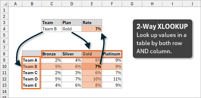
Basic 2-Way XLOOKUP Setup

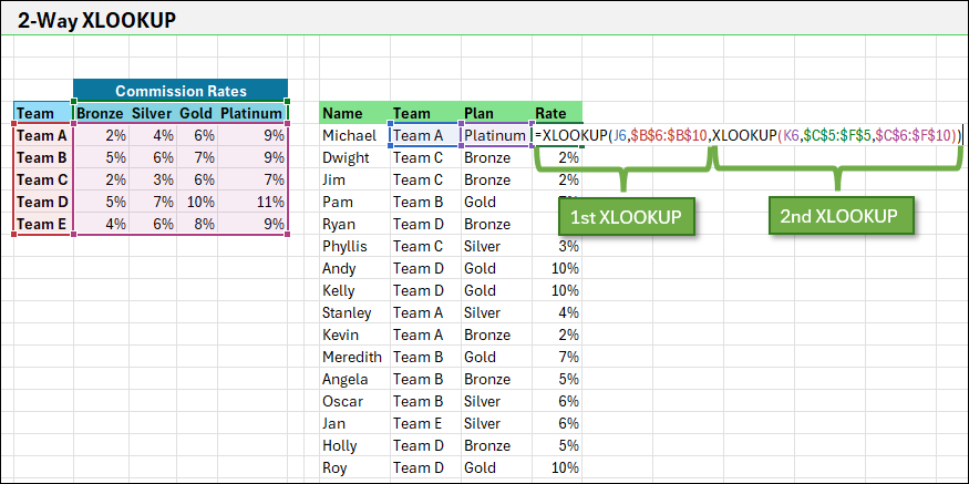
1. Starting with Rows: Using the data set provided in the file above, begin by typing =XLOOKUP( and setting your team (row) as the lookup value. Select your row range, and press F4 to lock the range.
2. Adding Columns: Next, nest another XLOOKUP to handle the plan (column) lookup by selecting the plan header row and applying F4 to anchor it.
3. Final Return Array: For the return array, select the entire range of values in the source data to allow dynamic row/column results, providing an efficient way to cross-reference values.

Your formula should look something like this:

=XLOOKUP(J6,$B$6:$B$10,XLOOKUP(K6,$C$5:$F$5,$C$6:$F$10))

---

Advanced Error Handling with 2-Way XLOOKUP

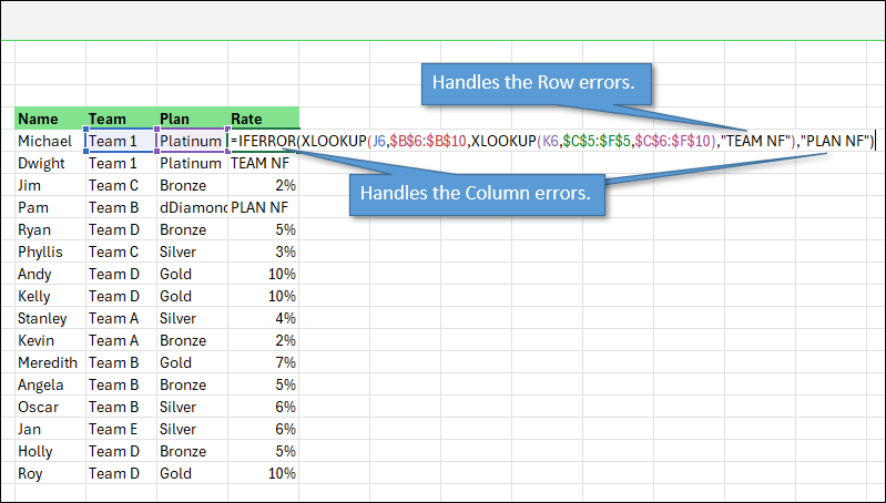
Handling errors effectively in a 2-way XLOOKUP setup requires managing both row and column lookups separately, allowing you to see exactly which part of the lookup is causing an issue. Here’s how you can achieve this with two different approaches:

1. Error Handling for Row Lookup (Team Not Found):
   If the team name you’re trying to look up doesn’t exist in the data, Excel would return an error. By adding if_not_found to the first XLOOKUP (the row lookup), you can set up a custom error message that clearly indicates the issue is with the row.
   • For example, append , "Team NF" to the end of the row lookup within the XLOOKUP function. Here, “Team NF” stands for “Team Not Found” and will appear any time the lookup value in the team row isn’t present.
2. Error Handling for Column Lookup (Plan Not Found):
   Unlike the row lookup, if the plan you’re referencing isn’t available, the entire XLOOKUP will still attempt to complete. Since this component doesn’t use the if_not_found argument, wrap this part of the formula in an IFERROR statement. This way, if the XLOOKUP can’t find the specified column header, it will display a custom error for the plan.
   • For example, IFERROR(XLOOKUP(...), "Plan NF") will ensure the formula returns “Plan NF” for a missing plan, giving you separate, specific messages for missing rows or columns.

This handling provides clear error messages that show where the data retrieval issue lies, making it easier to diagnose and resolve mismatches in your data.

---

Working with Excel Tables

Switching your data to Excel tables can automate formula management. Instead of fixed ranges, reference the header row and entire table to keep formulas dynamic as the table grows.

Using Excel Tables, our formula would look something like this:

=XLOOKUP([@Team],tblRate[Team],XLOOKUP([@Plan],tblRate[#Headers],tblRate))

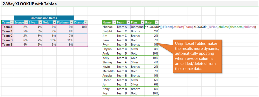
For more information on how to get started using Excel Tables, check out this tutorial: Excel Tables Tutorial Video – Beginners Guide for Windows & Mac

---

Using XLOOKUP for Range Lookups (Closest Match)

For lookups where you need to find a value within a range rather than an exact match, XLOOKUP’s Closest Match option offers a solution. This is particularly useful in tier-based data, where the exact lookup value may not exist in the dataset but should fall within a specific range.

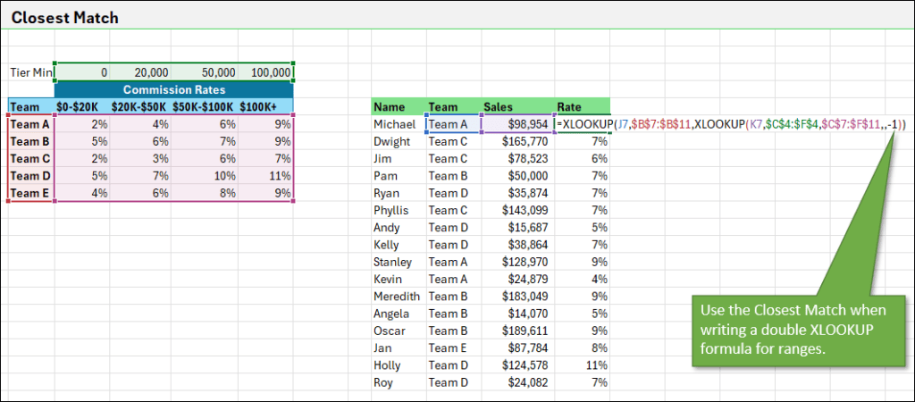
In this scenario, set up your data to have tier minimums in a separate row to act as lookup references. For example, if you’re working with sales ranges, the tier minimums row might include values like 0, 20,000, 50,000, and so on.

• Step-by-Step for Closest Match:
  • Step 1: Begin with your primary XLOOKUP for the row (e.g., team) and select the tier minimums row as the array for the column XLOOKUP.
  • Step 2: Instead of an exact match, use match_mode = -1 for Next Smaller Item. This tells Excel to return the closest, smaller tier when the exact match isn’t available. For example, if you’re looking up a sales value of 98,000, the formula will find the tier below it (50,000) if an exact match doesn’t exist.

This ensures the lookup references the appropriate range and calculates the corresponding value accurately. It’s especially helpful when ranges are large or data is not in strict order, as XLOOKUP can manage unordered lists and still retrieve the correct range.

Here's how the formula looks for our example:

=XLOOKUP(J7,$B$7:$B$11,XLOOKUP(K7,$C$4:$F$4,$C$7:$F$11,,-1))

---

Comparing XLOOKUP with INDEX MATCH

While both 2-way XLOOKUP and INDEX MATCH offer similar results, XLOOKUP has:

• Fewer functions, making it simpler to write and troubleshoot.
• Superior error-handling capabilities, allowing specific error messages for rows and columns separately.

If you'd like to learn more about how INDEX MATCH works, watch this video: How to Use Index Match Instead of Vlookup

---

Practice Challenge

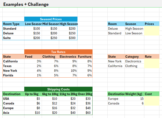
Finally, test your skills with this 2-way XLOOKUP practice challenge. Download the Excel file [EMBED] and try writing formulas to complete each example.

Conclusion

Using a 2-way XLOOKUP formula enables you to look up complex data efficiently. This tutorial covered basics to advanced applications, equipping you to handle real-world scenarios in Excel. Leave a comment and let us know how you’re applying this technique!

Black Friday Offer – Modern Formulas