Comparative Distribution Chart – Histogram or Box Plot Alternative

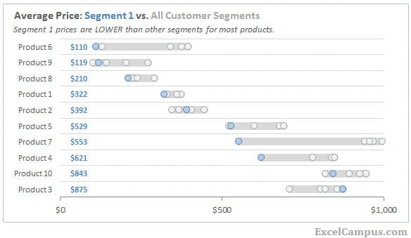
It can be difficult to create visualizations that compare one segment against an entire population of data while displaying the distribution of the entire population.  In this post I'm going to explain how to create the following chart in Excel.  

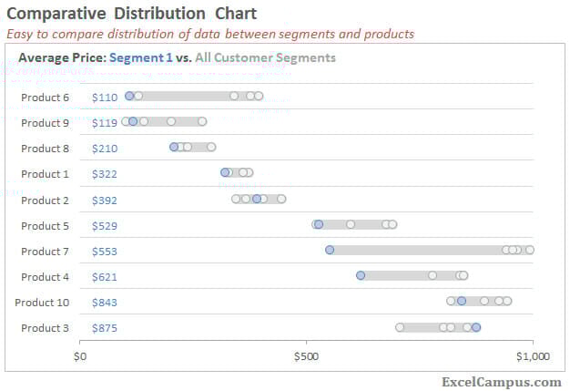
In this case we want to see pricing distribution for several products by customer segment.  So the data values are average price, and the categories are the products and customer segments.  But this same technique could be used for any combination of data value and categories; sales by product and region, headcount by department and country, etc.

The Challenge

I was recently doing analysis on product pricing data and the goal was to determine how one customer segment was performing against all the rest.  How does the the average price of each product in Segment 1 compare to the rest?  Like all good charting or data visualization projects, it took many iterations to come up with a chart that clearly communicated the story without too much explanation.  

Alternative 1: Box Plot or Quartile Plot

I first started with the box plot or quartile plot.  This is a great way to see the distribution of your data and compare it to other segments or categories.  The major issue I had with the box plot is that not everyone understands it.  So the use of a box plot depends on your audience.  If the audience is familiar then it is a great solution.  However, trying to explain it can be time consuming and not worth the effort.

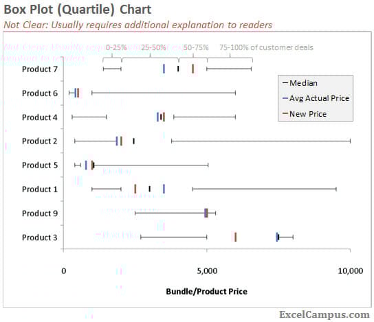
Box plots also work well if you have a large number of segments/categories.  In the comparative distribution chart we are only looking at 5 different customer segments.  If you had hundreds or thousands of segments, then the box plot is probably a better solution.  I will explain how I created it in a separate post.  If you want a hint, it's actually a line chart turned on its side.

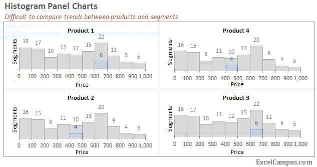
Alternative 2: Histograms

Histograms are a good alternative for a single category, but comparing multiple categories doesn't really work.  You could combine several histograms into a panel chart, but it is hard to identify trends between categories.

How to Create the Comparative Distribution Chart

There are two files you can download below that will help guide you through creating this type of chart.  

• The “Comparative Distribution Chart Guide.xls” file contains a detailed step-by-step guide.  
• The “Comparative Distribution XY Chart.crtx” file is a Chart Template file that you can use to change the chart type to resemble the comparative distribution chart.  This will save you a lot of time in formatting the chart.

Step 1 

Your original data should look similar to the format below, with products in each row and columns for each segment.  Using a pivot table to summarize your raw data would be an easy way to get the data in this format.  

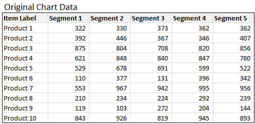
Once you have the data table, then you need to add a few columns that will be used to plot the points in the XY Scatter chart.  I've added cell notes in the guide file that give more detail on the calculations in each column. 

Step 2

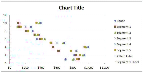
Create the XY Scatter chart and add all the data series.  It's best to select a blank cell and then insert the “Scatter with Only Markers” chart type.  Then add each data series individually.  Excel has a tough time trying to automatically figure out the X and Y values for each series if you try to select the whole table and create the chart.  So it's best to add each series one-by-one.

Note: You can skip steps 3 and 4 below by applying the Comparative Distribution XY Chart template.  This will automatically do all the formatting for you.

Step 3

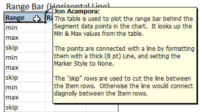
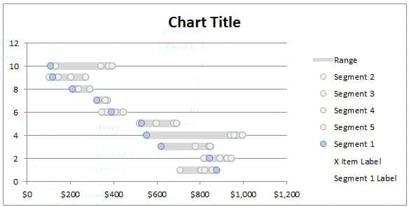
Now that you have all the series plotted on the chart, you need to format the marker options and line colors/styles for each series.  You'll want each series to have the same marker style and color except for the series you are comparing.  In this case we want Segment 1 to have blue circle markers, and all other segments to be gray.  The Range Bar series is the light gray background bar that shows the range from min to max for each product.  For this series, set the markers to None, and change the line style width to 8.5pt.  This will create a thick line in the background.  You may also have to rearrange the order of your series if the background bar is on top of the other points.

Step 4

The chart axes need to be changed so the data points are plotted between the horizontal grid lines.  The vertical axis needs to be changed by starting the minimum axis at 0.5 and changing the major unit to 1.0 on the vertical axis.

You can also change the major units on the horizontal axis to reduce the clutter.  We really only need to see the min and max values and maybe a few points in between to give some scale to the chart.

Step 5

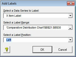
Add labels for the product and Segment 1 price.  The fastest and easiest way to do this is by using the XY Chart Labels add-in.  It's available for free download and very easy to use.

http://www.appspro.com/Utilities/ChartLabeler.htm

Step 6

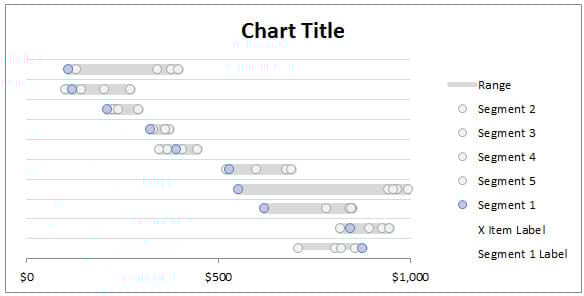
Finally, put some finishing touches on your chart to make it look presentable.  Tuck in its shirt and comb its hair. 🙂  And basically remove all the unnecessary chart junk that is not needed to tell the story.  We are trying to clearly show how Segment 1 compares to the other segments across all product lines.  

Pros and Cons

Pros

The comparative distribution chart combines a little bit of both the box plot and simple histogram.  With the added bonuses of being easy to explain, and allowing for comparison of one data point against the whole data set.  It's use will depend what trends or messages the chart clearly conveys to the reader.  In this case the Segment 1 prices are lower than the others for almost every product.  That would be a clear indication that Segment 1 has some defining characteristics that create this behavior.  Possibly, Segment 1 customers always use coupons that other segments don't have access to.  

Cons

This chart is best for small number of segments.  If we had 50 customer segments instead of 5, then it would be difficult to see the distribution of all the data points in the range for each product.  A box plot would be better suited for this.

Download

This model could be further enhanced by adding a drop-down to select the segment you want to compare to the others.  I'm sure you will find many possibilities for modifying it.

Please let me know if you have any questions.  I'd like to hear how you could use this or improve on it.  Thanks!