Bottom line: Take on this Excel challenge to convert text to time values.
Skill level: Intermediate
Video Explanation
Download the Excel File
You can download the Excel file that contains the data for the challenge below.
The Challenge
This challenge was based on a question from Mark, a member of the Excel Campus community. He exports a report from their training system that contains a column with the total amount of training time that each employee has completed.
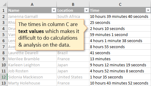
The problem is that the time is a text value written in the following format.
## hour(s) ## minute(s) ## second(s)
The values are NOT recognized by Excel as a date/time data type. This makes it very difficult to do any type of calculations and analysis on the data.
For example, we might want to see a summary report with the average time spent by Location. That will be very easy to create once the data is cleaned up.
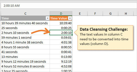
So the challenge is to convert the text values into time values that Excel recognizes.
The Rules
There are only two simple rules for this challenge:
- You can use any Excel tools/features you'd like (formulas, Power Query, VBA, etc.).
- The cells with the results must contain time values. See this article on the Date System in Excel for further explanation.
Share Your Solution
Please leave a comment below (or on the YouTube video) that explains your solution.
You can also upload your solution file to a cloud sharing service (OneDrive, Google Drive, Dropbox) and share the link.
Note: After you leave a comment below you might not see it on the post right away. It takes time to be approved and clear the site cache.
A Great Learning Opportunity
I'm excited to see your solution, and believe this will be a great way for us to all learn from each other.
Here are links to the solution posts where I explain a few popular techniques for converting text to time.
- Convert Text to Time Values with Formulas
- Convert Text to Time Values with Power Query
- Convert Text to Time Values with UDFs in VBA
Thanks again and have a nice day! 🙂


A formula works well in this situation:
=IFERROR(TRIM(LEFT([@Time],FIND(“h”,[@Time],1)-1)),0)&”:”&IFERROR(MID([@Time],FIND(“m”,[@Time],1)-3,2),”00″)&”:”&IFERROR(MID([@Time],FIND(“se”,[@Time],1)-3,2),”00″)
Peter
Brute force always works for me…. 🙂
=VALUE(TEXT(IFERROR(LEFT([@Time],FIND(“h”,[@Time],1)-2),”0″)&”:”&IFERROR(MID([@Time],FIND(“m”,[@Time],1)-3,2),”00″)&”:”&IFERROR(MID([@Time],FIND(“c”,[@Time],1)-5,2),”00″),”h:mm:ss”))
Find and replace all (Minutes,seconds,hour) characters to “:”
it will automatically convert to time , if not – use formula = TIME(Refernce cell)
Nice one, you are genius!!!
=CONCAT(IFERROR(VALUE(MID(C2,1,SEARCH(“hours”,C2)-1)),0),”:”,(IFERROR(VALUE(MID(C2,MAX(SEARCH(“minutes”,C2)-3,1),2)),0)),”:”,(IFERROR(VALUE(MID(C2,MAX(SEARCH(“seconds”,C2)-3,1),2)),0)))
Glad I am not the only one, 😉
Jerry’s way, take 2
i.e.
don’t force it, get a bigger hammer
=TIME(IFERROR(TRIM(MID([@Time];MAX(1;FIND(” h”;[@Time])-2);2));0);IFERROR(TRIM(MID([@Time];MAX(1;FIND(” m”;[@Time])-2);2));0);IFERROR(TRIM(MID([@Time];MAX(1;FIND(” s”;[@Time])-2);2));0))
A good challenge to get my brain going this morning.
Similar to what was already posted:
=TIME(
IF(ISERR(SEARCH(“hour”,C101)>0),0,LEFT(C101,2)),
IF(ISERR(SEARCH(“minute”,C101)>0),0,MID(C101,SEARCH(“minute”,C101)-3,2)),
IF(ISERR(SEARCH(“second”,C101)>0),0,MID(C101,SEARCH(“second”,C101)-3,2))
)
Format cell as h:mm:ss
As it turned out my proposal had slight variations in columns D:F as compared to ‘Solution’ sheet.
D: =IFERROR(VALUE(MID(C2,SEARCH(D$1,C2)-(SEARCH(D$1,C2)-1),2)),0)
E: =IFERROR(VALUE(MID(C2,SEARCH(E$1,C2)-(MIN(SEARCH(E$1,C2)-1,3)),2)),0)
F: =IFERROR(VALUE(MID(C2,SEARCH(F$1,C2)-3,2)),0)
Formula for column G was the same.
I hope that you have a blessed day.
Got there in the end. Didn’t think to put hour minute second headings in top line, that would have made it shorter. Or to format data as a table, always seem to forget that. 🙂
VBA brute force:
Option Explicit
Function GetTime(ByVal s As String) As Double
GetTime = Evaluate(Replace(Replace(Replace(Replace(Replace(s, ” hour”, “*1/24″), ” minute”, “*1/24/60″), ” second”, “*1/24/60/60”), “s”, “”), ” “, “+”))
End Function
Just convert the string into a calculation and evaluate it…
Nifty detail: make sure singular and plural of “hour”, etc. are both treated.
Hi there!,
I just used the following formula as a way on converting it into a string with the appropriate format: (the target cell is c2). It looks for hour, minute and second and inputs an appropriate string using iferror(). Excel properly interpreted it as a time field without any celll formatting applied.
=RIGHT(TRIM(“00″&IFERROR(LEFT(C2,FIND(“hour”,C2)-2)&”:”,”00:”)),3)&RIGHT(“00″&TRIM(IFERROR(MID(C2,FIND(“minute”,C2)-3,2)&”:”,”00:”)),3) & RIGHT(“00″&TRIM(IFERROR(MID(C2,FIND(“second”,C2)-3,2),”00″)),2)
I like yours best so far, taking advantage of how Excel nowadays thinks of any number-looking thing as precisely what it looks like to be able to use a simpler formula. Tres clever.
I don’t see how TRIM() is required, considering the “00” present for each.
Also, I’d still wrap a TIMEVALUE() on it for formatting and to ensure it works as input for most anything or anyone.
This formula seems to cover all possibilities. The text is in cell A1 and I’ve put the formula in cell B1, which is formatted as “h:mm:ss”:
=TIME(IFERROR(IFERROR(VALUE(MID($A1,(FIND(“h”,$A1)-3),2)),VALUE(MID($A1,(FIND(“h”,$A1)-2),1))),”00″),IFERROR(IFERROR(VALUE(MID($A1,(FIND(“m”,$A1)-3),2)),VALUE(MID($A1,(FIND(“m”,$A1)-2),1))),”00″),IFERROR(IFERROR(VALUE(MID($A1,(FIND(“sec”,$A1)-3),2)),VALUE(MID($A1,(FIND(“sec”,$A1)-2),1))),”00″))
The TIME formula takes the arguments (hours, minutes, seconds). The first IFERROR is checking to see if “h”, “m” or “sec” are found in the text. If they are not there, it defaults the value to “00”. If found, the 2nd IFERROR is used to distinguish between single digit and double digit hours, minutes or seconds.
These are some examples of the results:
2 hours 3 minutes 40 seconds 02:03:40
12 hours 17 minutes 3 seconds 12:17:03
17 minutes 12 seconds 00:17:12
3 hours 03:00:00
55 seconds 00:00:55
[Blank] 00:00:00
=TIMEVALUE(IFERROR(LEFT(C2,FIND(“hours”,C2)-2),”00″)&”:”&IFERROR((MID(C2,FIND(“minutes”,C2)-3,2)),”00″)&”:”&IFERROR(MID(C2,FIND(“seconds”,C2)-3,2),”00″))
Use FIND to get the position for each of hours, minutes, seconds
Use LEFT to get the number text to the left of hours
Use MID to get the number text to the left of minutes and seconds
Use IFERROR to determine if something’s not found and replace it with 00
Use concatenation to insert “:” between the text values found of hours, minutes and seconds
Use TIMEVALUE to convert the text to a time
Format the cell as [h]:mm:ss
David,
You solution needs to be tweaked a little. Not all of the times are plural so where they are not, you will return an incorrect 00 value. Look at your value for seconds in row five for example. Change your formulas to look for the singular value of the word and you will be 100% correct.
Ex: Change “seconds” to “second” or just “s”
Thanks Jeffrey. Good catch.
Here’s my revised formula; I added the VALUE function so the value returned is formatted by this formula.
=VALUE(TEXT(TIMEVALUE(IFERROR(LEFT(Table1[@Time],FIND(“hour”,Table1[@Time])-2),”00″)&”:”&IFERROR((MID(Table1[@Time],FIND(“minute”,Table1[@Time])-3,2)),”00″)&”:”&IFERROR(MID(Table1[@Time],FIND(“second”,Table1[@Time])-3,2),”00″)),”[h]:mm:ss”))
Hello David,
I like the approach. However this solution fails where there is a single hour, minute or second which can be resolved by replacing “hours” with “hour”, “minutes” with “minute” and “seconds” with “second” in your formula.
This corrected most lines but left an issue with cases with “no hours AND under 10 minutes” or “no hours and/or minutes AND under 10 seconds”. I think this addition to your formula (below) will work in all cases.
=TIMEVALUE(IFERROR(LEFT(C2,FIND(“hour”,C2)-2),”00″)&”:”&IFERROR((MID(C2,MAX(1,FIND(“minute”,C2)-3),2)),”00″)&”:”&IFERROR(MID(C2,MAX(1,FIND(“second”,C2)-3),2),”00″))
See row with 727 “1 minute 54 seconds” for best example of where formulas differ.
Regards,
Vincent
Split the date using TextToColumns with space as the delimiter. Then us this formula to reate times
=TIMEVALUE(TEXTJOIN(“:”,FALSE,IF(ISBLANK(C2),0,C2),IF(ISBLANK(E2),0,E2),IF(ISBLANK(G2),0,G2)))
Copy paste as value and format as Time. Remove columns that are not required
I don’t think this works. Since every input time doesn’t contain all the units (hours/minutes/seconds), using TextToColumns doesn’t automatically put the right values in the right columns. For example, this turns row 3 into 25 hours, not 25 seconds.
Ciao Jon, herewith my PQ solution:
https://drive.google.com/drive/folders/1n5m2azfBl3ikmWP1LQDLilXhEYChzaf9?usp=sharing
Hour Column: =IFERROR(LEFT(C2,FIND(“hour”,C2)-1),”00″)
Minutes Column: =IFERROR(MID(C2,FIND(“minute”,C2)-3,2),”00″)
Seconds Column: =IFERROR(MID(C2,FIND(“second”,C2)-3,2),”00″)
Time Value Column: =TIME(D2,E2,F2)
Copy D2, E2, F2 and G2 to the bottom
=TIME(IFERROR(TEXT(MID(C2,1,FIND(” hours”,C2,1)-1),”00″),0),IFERROR(TEXT(MID(C2,FIND(“minutes”,C2,1)-3,2), “00”), 0),IFERROR(TEXT(MID(C2,FIND(“seconds”,C2,1)-3,2), “00”), 0))
Not sure if it’s the best way.
Very interesting exercise! Thanks Jon!
I favor formulas over macros. But I went the macro route here. It works. And could also benefit from further optimization.
Function FixCustomTime(ByVal sTime As String) As Double
sTimesArray = Split(sTime, ” “)
sHour = “00”
sMinute = “00”
sSecond = “00”
i = 0
Do While i <= UBound(sTimesArray)
sValue = sTimesArray(i)
sLabel = sTimesArray(i + 1)
If InStr(sLabel, "hour") 0 Then
sHour = Right(“0” & sValue, 2)
End If
If InStr(sLabel, “minute”) 0 Then
sMinute = Right(“0” & sValue, 2)
End If
If InStr(sLabel, “second”) 0 Then
sSecond = Right(“0” & sValue, 2)
End If
i = i + 2
Loop
FixCustomTime = TimeValue(sHour & “:” & sMinute & “:” & sSecond)
End Function
Hi,
Here my solution, using columns E, F and G as intermediate calculations cells for the extractions of hours, minutes and seconds respectively, and concatenating the partial results in column D :
Hours (E2) :
=IFERROR(IF(FIND(“hours”;C2);LEFT(C2;2));0)
Minues (F2):
=IFERROR(IF(FIND(“minutes”;C2);MID(C2;FIND(“minutes”;C2)-3;2));0)
Seconds (G2):
=IFERROR(IF(FIND(“seconds”;C2);MID(C2;FIND(“seconds”;C2)-3;2));0)
Time (D2):
=(E2*3600+F2*60+G2)/86400
https://wmfexcel.com/2016/02/20/make-impossible-possible/
This is my formula approach.
A Power Query solution in 12 steps and no “M” code. All done with PQ user interface and built in functions.
https://1drv.ms/x/s!AiCGN7G0L7PalAIspV6SXoIStYG4
Thanks, great example !
Kirk, what version of Excel are you using? My installation says that yours is newer and it’s using at least 1 Power Query function that I don’t have.
James
I’m using Excel 2016
I was able to complete the challenge using text to columns and 3 nested IF statements.
Here is a power query approach which uses the advance settings in the “text before delimiter” and “text between delimiter” functions.
As the last step after loading to an excel table change the formatting to time without the am/pm reference.
let
Source = Excel.CurrentWorkbook(){[Name=”Table1″]}[Content],
#”Lowercased Text” = Table.TransformColumns(Source,{{“Time”, Text.Lower, type text}}),
#”Trimmed Text” = Table.TransformColumns(#”Lowercased Text”,{{“Time”, Text.Trim, type text}}),
GetHours = Table.AddColumn(#”Trimmed Text”, “Hours”, each Text.BeforeDelimiter([Time], ” hour”, {0, RelativePosition.FromEnd}), type text),
GetMins = Table.AddColumn(GetHours, “Minutes”, each Text.BetweenDelimiters([Time], ” min”, ” “, {0, RelativePosition.FromEnd}, {0, RelativePosition.FromEnd}), type text),
GetSecs = Table.AddColumn(GetMins, “GetSecs”, each Text.BetweenDelimiters([Time], ” sec”, ” “, {0, RelativePosition.FromEnd}, {0, RelativePosition.FromEnd}), type text),
ReplaceBlanks = Table.ReplaceValue(GetSecs,””,”0″,Replacer.ReplaceValue,{“Hours”, “Minutes”, “GetSecs”}),
MergeHMS = Table.CombineColumns(ReplaceBlanks,{“Hours”, “Minutes”, “GetSecs”},Combiner.CombineTextByDelimiter(“:”, QuoteStyle.None),”Time Value”),
#”Changed Type” = Table.TransformColumnTypes(MergeHMS,{{“Name”, type text}, {“Location”, type text}, {“Time”, type text}, {“Time Value”, type time}})
in
#”Changed Type”
Very Nice! Just wish that the quotation marks would copy directly so that they don’t all have to be changed to see this work.
Here is the link to the text file that contains the M code above since the comment system is causing issues with quotes.
https://docs.google.com/document/d/1zkWrI-lGs5chxX8Ka0ayOEg7TwSy5BvSfxHyNrXkvTw/edit?usp=sharing
There is no custom M code just using built in power query functions from the top menu.
Here is my video solution using text to columns and nested IF statements
https://youtu.be/D9FtYZaSUnM
First, convert “Text to Columns” using Space and “s” as delimiters. I had the new values written into “Column1” through “Column6”. Since the formatting is inconsistent, we then need to look for the right values to construct our time. Using the “s” as a delimiter simplifies this slightly because it removes the ambiguity about single vs plural units.
For the hours, you only need to look in the first pair of columns. For minutes, you need to look in the first and second pair of columns. For seconds, you need to look in all three.
=TIME(
IF([@Column2]=”hour” ,[@Column1],0),
IF([@Column2]=”minute”,[@Column1],IF([@Column4]=”minute”, [@Column3],0)),
IF([@Column2]=”econd” ,[@Column1],IF([@Column4]=”econd” ,[@Column3],[@Column5]))
)
I used this formula:
=TIME(
IFERROR(IF(SEARCH(“hour”,[@Time],1)=4,MID([@Time],SEARCH(“hour”,[@Time],1)-3,2),MID([@Time],SEARCH(“hour”,[@Time],1)-2,2)),0),
IFERROR(IF(SEARCH(“minute”,[@Time],1)=3,MID([@Time],SEARCH(“minute”,[@Time],1)-2,2),MID([@Time],SEARCH(“minute”,[@Time],1)-3,2)),0),
IFERROR(MID([@Time],SEARCH(“second”,[@Time],1)-3,2),0))
It looks better when separated by enter breaks.
The other not so elegant, but fast solution would be using Find And Replace to change all “hours”,”minutes”, and “seconds” to “:”
Would prefer “Search” over “Find” to avoid case sensitivity.
=SUBSTITUTE(IFERROR(MID(C2,MAX(1,SEARCH(“h”,C2)-3),2),0)&”:”&IFERROR(MID(C2,MAX(1,SEARCH(“m”,C2)-3),2),0)&”:”&IFERROR(MID(C2,MAX(1,SEARCH(“se”,C2)-3),2),0),” “,””)+0
I used helper columns to find the “Hour”, “Minute”, “Second” and find where the beginning respective number is and if not present, =0. I then used Time function to convert to time.
I used search and Mid too.
Not as difficult as I thought.
This was great! I went the route of figuring out how many seconds there are total, and this returns the time value # which can be formatted as h:mm:ss.
=SUMPRODUCT(VALUE(IFERROR(MID(0&[@Time],FIND({“h”,”m”,”sec”},0&[@Time])-3,2),{0,0,0})),{3600,60,1})/86400
I produced a UDF to add to my personal workbook. I also wrote it so that it could be easily adapted to used for other data types e.g. 5 years 6 months 2 days
It’s a bit messy and I may have to tidy up all the if statements, but it seems to work.
Option Explicit
Const DATA_STRING_HOUR = “Hour”
Const DATA_STRING_MINUTE = “Minute”
Const DATA_STRING_SECOND = “Second”
Private Function Extract(ByVal strMyTime As String, strTimePart As String) As Long
strMyTime = LCase(strMyTime)
strTimePart = LCase(strTimePart)
Dim lngPosStart As Long
Dim lngPosEnd As Long
lngPosEnd = InStr(1, strMyTime, strTimePart)
If lngPosEnd 0 Then
lngPosStart = InStrRev(strMyTime, ” “, lngPosEnd – 2)
Else
lngPosStart = 1
End If
If lngPosStart = 0 Then
lngPosStart = 1
End If
If lngPosEnd 0 Then
Extract = CLng(Trim(Mid(strMyTime, lngPosStart, lngPosEnd – lngPosStart)))
End If
End Function
Function ExtractTime(ByVal strMyTime As String) As Date
Dim lngHour As Long
Dim lngMinute As Long
Dim lngSecond As Long
lngHour = Extract(strMyTime, DATA_STRING_HOUR)
lngMinute = Extract(strMyTime, DATA_STRING_MINUTE)
lngSecond = Extract(strMyTime, DATA_STRING_SECOND)
ExtractTime = TimeSerial(lngHour, lngMinute, lngSecond)
End Function
1. Created 3 coloumns for individual segments:
=IFERROR(IFERROR(MID(C2,FIND(“hour”,C2,1)-3,2),MID(C2,FIND(“hour”,C2,1)-2,2)),0)
2. And then merged results using:
=TEXTJOIN(“:”,TRUE,D2:F2)
I went old school. Converted text into columns using ‘space’ as Delimiter, sorted first word column for hours, inserted cells to shift non Hour entries left, sorted next word column for Seconds, inserted cells to shift non Seconds entries to the left.
End result = 6 columns:
[XXX] [Hours] [XXX] [Minutes] [XXX] [Seconds]
Time formula then combined data into one time
Custom number format applied
Done.
Used this to make a formula string in cell D2 and copied down column D
=IF(NOT(ISERROR(FIND(“econd”,SUBSTITUTE(C2,”s”,””),1))),
IF(NOT(ISERROR(FIND(“minute”,SUBSTITUTE(C2,”s”,””),1))),
SUBSTITUTE(SUBSTITUTE(SUBSTITUTE(SUBSTITUTE(C2,”s”,””),” econd”,”/86400″),” minute “,”/1440+”),” hour “,”/24+”),
SUBSTITUTE(SUBSTITUTE(SUBSTITUTE(C2,”s”,””),” econd”,”/86400″),” hour “,”/24+”)),
IF(NOT(ISERROR(FIND(“minute”,SUBSTITUTE(C2,”s”,””),1))),
SUBSTITUTE(SUBSTITUTE(SUBSTITUTE(C2,”s”,””),” minute”,”/1440″),” hour “,”/24+”),
SUBSTITUTE(SUBSTITUTE(C2,”s”,””),” hour”,”/24″)))
Then used “Named Range” trick at this link to use the “Hidden EVALUATE” formula.
https://www.myonlinetraininghub.com/excel-factor-12-secret-evaluate-function
And formatted result as time.
An unusual approach but may be useful to know these tricks one day.
Hi,
it seems the format is not fixed x hour(s) y minute(s) z second(s) but if the numerical values are 0, that part of the format does not appear.
Meaning the formulation of the problem is not entirely correct.
Because otherwise you would expect in row 3 this :
0 hours 0 minutes 25 seconds
for example
Otherwise I would have gone for the replacement approach as well. Replacing the spaces with colons is nice to then be able to have Excel interpret it as time.
I have concluded formula as below.
TIME(IFERROR(REPLACE(C2, FIND(” hour”, C2, 1),30,””), “”), IFERROR(RIGHT(REPLACE(C2, FIND(” minute”, C2, 1),30,””), 2), “”), IFERROR(RIGHT(REPLACE(C2, FIND(” second”, C2, 1),30,””), 2), “”))
Nice solution but:
Replace the IFERROR ”” by 0
TIME(IFERROR(REPLACE(C2, FIND(” hour”, C2, 1),30,””), 0),
IFERROR(RIGHT(REPLACE(C2, FIND(” minute”, C2, 1),30,””), 2), 0),
IFERROR(RIGHT(REPLACE(C2, FIND(” second”, C2, 1),30,””), 2), 0))
After converting text to columns, I used a lookup table that shows the number of seconds for an hour and minute. The sum of the seconds for each of the three fields yields a total number of seconds that can then be converted into a time value.
The key to converting the text to seconds is in the following lookup formula: =IFERROR([@Time]*VLOOKUP([@Column2],$M$28:$N$34,2,TRUE),0)+IFERROR([@Column3]*VLOOKUP([@Column4],$M$28:$N$34,2,TRUE),0)+IFERROR([@Column5]*VLOOKUP([@Column6],$M$28:$N$34,2,TRUE),0)
The IFERROR accounts for lines with fewer than all three time designations.
Note the lookup table needs to include “hours” and “hour,” “minutes” and “minute,” etc.
I went back to basics and did a simple text to columns producing 6 columns then I did an auto filter on the all columns – then filtered the last column which only contained the words “seconds”, “second” or “blank. I chose to filter for “second” and “seconds” only (not blank). this resulted in all my columns
sorting all the hour into one column minutes into one column etc. I then used the time function to convert the 3 numerical columns into the correct format.
One more step was necessary to complete all lines….I had to go back and unfilter the columns and copy the formula down for all the rows that did not have seconds..
I used Power Query also, but was unable to figure out how to do it without custom M code.
I used the VBA Split function in a UDF which creates a pair of elements for each of hour, minute or second that may be present.
hours if column C contains “hour” then extract the first 2 digits, otherwise return “00”
=IF(ISNUMBER(SEARCH(“hour*”,[@Time])),LEFT([@Time],2),”00″)
minutes find “m” in column C, move back 3 spaces and extract 2 digits; wrapped in an ‘IFERROR’ to return “00”
=IFERROR(MID([@Time],FIND(“m”,[@Time])-3,2),”00″)
secs find “sec” in column C, move back 3 spaces and extract 2 digits; wrapped in a ‘IFERROR’ to return “00”
=IFERROR(MID([@Time],FIND(“sec”,[@Time])-3,2),”00″)
duration textjoin the three columns with “:” as the delimiter, wrapped in a TEXT function formatted as HH:MM:ss
=TEXT(TEXTJOIN(“:”,TRUE,[@Hours],[@Min],[@Sec]),”HH:MM:ss”)
Here is a link to my solution.
http://bit.ly/2W4F8cK
I have updated my solution because when I was extracting the minutes I did not allow for cells that contained no hours and only single digit minutes.
hours: if column C contains “hour” then extract the first 2 digits, otherwise return “00”
formula: =IF(ISNUMBER(SEARCH(“hour*”,[@Time])),LEFT([@Time],2),”00″)
minutes: if the string “hour” does not exist in column C then extract the first two digits, else find “m”, move back 3 spaces and extract 2 digits
formula: =IF(NOT(ISNUMBER(SEARCH(“hour”,@Time]))),LEFT([@Time],2),MID([@Time],FIND(“m”,[@Time])-3,2))
secs: find “sec” in column C, move back 3 spaces and extract 2 digits; wrapped in a ‘IFERROR’ to return “00”
formula: =IFERROR(MID([@Time],FIND(“sec”,[@Time])-3,2),”00″)
duration: textjoin the three columns with “:” as the delimiter, wrapped in a TEXT function formatted as HH:MM:ss
formula: =TEXT(TEXTJOIN(“:”,TRUE,[@Hours],[@Min],[@Sec]),”HH:MM:ss”)
Link to my solution with notes.
http://bit.ly/2ZFBjwM
I used Power Query to split the column and give me helper columns. Loaded the query as a new table and created an hours column, a minutes column and a seconds column.
The formulas are nested IF statements to return the matching value.
Then I TEXTJOINED the three columns, formatted as HH:MM:ss
Then I hid the helper columns.
This approach allows for the fact the format in the original column is not always n hours, n minutes, n seconds.
Select sheet “Raw Data”
Run Macro SplitTextToTime
———————————————-
Sub SplitTextToTime()
Dim objRange1 As Range
Set objRange1 = Range(“C:C”)
” Clean everything after column C
Columns(“D:Z”).Select
Selection.Delete Shift:=xlToLeft
Range(“A1″).Select
” Headings
”Sheets(“xxxxxxxx”).Select
Range(“J1”).Select
ActiveCell.FormulaR1C1 = “Hours”
Range(“K1”).Select
ActiveCell.FormulaR1C1 = “Minutes”
Range(“L1”).Select
ActiveCell.FormulaR1C1 = “Seconds”
Range(“M1”).Select
ActiveCell.FormulaR1C1 = “Time”
Range(“J1:M1”).Select
With Selection
.HorizontalAlignment = xlRight
.VerticalAlignment = xlBottom
.Font.Bold = True
End With
Range(“A1″).Select
”SplitText
objRange1.TextToColumns _
Destination:=Range(“D1″), _
DataType:=xlDelimited, _
Tab:=False, _
Semicolon:=False, _
Comma:=False, _
Space:=True
”PlaceFormulas
[J2].Formula = “=IF(LEFT(E2,1)=””h””,D2,0)”
[K2].Formula = “=IF(LEFT(E2,1)=””m””,D2,0)+IF(LEFT(G2,1)=””m””,F2,0)”
[L2].Formula = “=IF(LEFT(E2,1)=””s””,D2,0)+IF(LEFT(G2,1)=””s””,F2,0)+IF(LEFT(I2,1)=””s””,H2,0)”
[M2].Formula = “=TIME(J2,K2,L2)”
Columns(“M:M”).Select
Selection.NumberFormat = “h:mm:ss”
Range(“M1″).Select
”CopyDownFormula
Dim Lastrow As Long
Lastrow = Range(“A1”).CurrentRegion.Rows.Count
Range(“J2:M” & Lastrow).FillDown
”OnlyValues
”Sheets(“xxxxxxx”).Select
Columns(“J:M”).Select
Selection.Copy
Range(“J1”).Select
Selection.PasteSpecial Paste:=xlPasteValues, Operation:=xlNone, SkipBlanks _
:=False, Transpose:=False
Application.CutCopyMode = False
Columns(“D:I”).Select
Range(“I1”).Activate
Selection.Delete Shift:=xlToLeft
Range(“A1”).Select
End Sub
Jon,
Very nice challenge.
On your possible solution (sheet “Solution”) is a small error.
If minutes or seconds are standing to teh left and has the value of 1 digit (1 – 9), the formula results in 0
See example row 172, 250, 405, 589, 667, 683, 727, 728, 741, 817, 837, 853, 878, 934, 965 and 970
5 minutes 55 seconds results in 0 0 55 00:00:55
In total you miss 74 minutes (seconds are correct: all values are between 10 – 60)
Nice weekend and greeting from The Netherlands
Hi Jon
I built this out in three separate columns (for testing and sanity), then combined them into one, and added the VALUE function to derive the time. C3 looks like this:
=VALUE(IF(ISERR(FIND(” hours”,C2)),”0:”,LEFT(C2,FIND(” hours”,C2)-1)&”:”) & IF(ISERR(FIND(” minutes”,C2)),”00:”,MID(C2,FIND(” minutes”,C2)-2,2)&”:”) & IF(ISERR(FIND(” seconds”,C2)),”00″,MID(C2,FIND(” seconds”,C2)-2,2)))
For really long data sets, this may get slow but at the size of the example it works pretty well. Converting this logic to VBA as a function would probably be better as the data sets get bigger.
great
=IFERROR(MID($B$6,SEARCH(“hours”,$B$6,1)-3,2),”00″)&”:”&IFERROR(MID($B$6,SEARCH(“minutes”,$B$6,1)-3,2),”00″)&”:”&IFERROR(MID($B$6,SEARCH(“seconds”,$B$6,1)-3,2),”00″)
this formula will produce the correct time format ie HH:MM:SS no matter what order the data is
Hi Jon.
My Power Query solution:
First split column by ” “.
Select columns Time.2, Time.4 and Time.6.
Replace “hour” with 24.
Replace “minute” with 1440.
Replace “second” with 86400.
Replace “s” with “”.
Change type to whole number.
Select columns Time.1 and Time.2.
Add column -> Division.
Select columns Time.3 and Time.4.
Add column -> Division.
Select columns Time.5 and Time.6.
Add column -> Division.
Select Division, Divison.1 and Divsion.3.
Add column -> Addition.
Remove all unnecessary columns.
Change type of column Addition to Time.
Change name of column Addition to Time Value.
Sorry people
i misinterpreted the challenge
My time, hrs, mins and sec, were all in same cell (C7)
Eg 11 hours 30 minutes 20 seconds
with the time in one cell, the below formula works
=IFERROR(MID($C$7,SEARCH(“hours”,$C$7,1)-3,2),”00″)&”:”&IFERROR(MID($C$7,SEARCH(“minutes”,$C$7,1)-3,2),”00″)&”:”&IFERROR(MID($C$7,SEARCH(“seconds”,$C$7,1)-3,2),”00″)