Bottom Line: Learn 4 different techniques for creating a list of numbers in Excel. These include both static and dynamic lists that change when items are added or deleted from the list.
Skill Level: Beginner
Watch the Tutorial
Download the Excel File
You can download the worksheet that I use in the video here:
Hidden Content
Numbered Lists
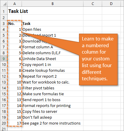
If you have a list of items in Excel and you'd like to insert a column that numbers the items, there are several ways to accomplish this. Let's look at four of those ways.
1. Create a Static List Using Auto-Fill
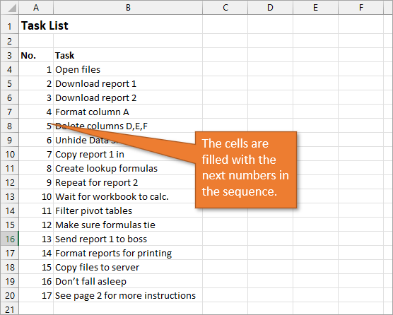
The first way to number a list is really easy. Start by filling in the first two numbers of your list, select those two numbers, and then hover over the bottom right corner of your selection until your cursor turns into a plus symbol. This is the fill handle.
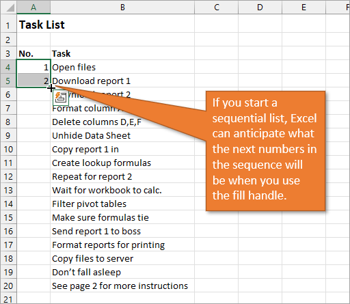
When you double-click on that fill handle (or drag it down to the end of your list), Excel will fill in the blanks with the next numbers in the sequence.
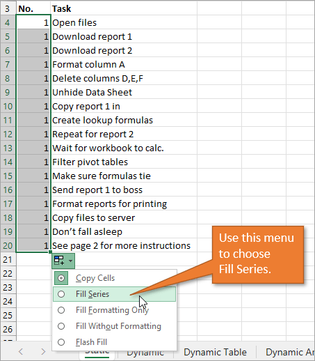
An alternate way to create this same numbered list is to type a 1 in the first cell and then double-click the fill handle. Because Excel doesn't have a second number to identify a sequence or pattern, it will fill down the columns with 1s. But you will notice that a menu is available at the end of your column, and from that menu, you can select the option to Fill Series. This will change the 1s to a sequential list of numbers.
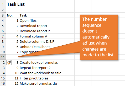
The numbered column we've created in both instances is static. This means it doesn't change when you make additions or deletions to the corresponding list of items. For example, if I insert a new row in order to add another task, there is a break in the numbered column as well, and I would have to repeat the same steps to correct the list.
So, unless we want the numbers to always remain as they are, a better option would be to create a dynamic list.
2. Create a Dynamic List Using a Formula
We can use formulas to create a dynamic list where the numbers update when we add or delete rows from the list.
To use a formula for creating a dynamic number list, we can use the ROW function. The ROW function returns the row number of a cell. If we don't specify a cell for ROW, it just returns the current row number of whatever is selected.
In our example, the first cell in our list doesn't start on Row 1. It starts on Row 4. But we don't want our list to start at 4; we want it to start at 1. To subtract the extra 3, our formula will include a minus sign and then the ROW function again, but this time pointed to the cell above our formula (which is in Row 3).
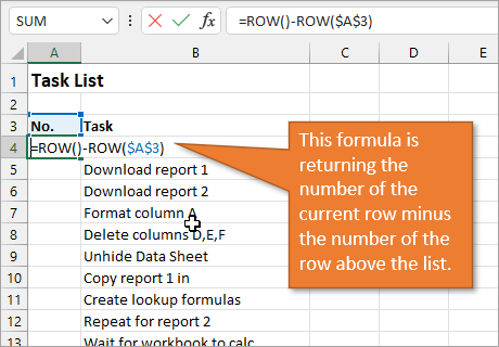
We use the absolute values (dollar signs) in our cell selection because we don't want that number to change as we copy the formula down the list. In other words, we always want to subtract 3 from the row number to give us our list number.
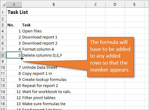
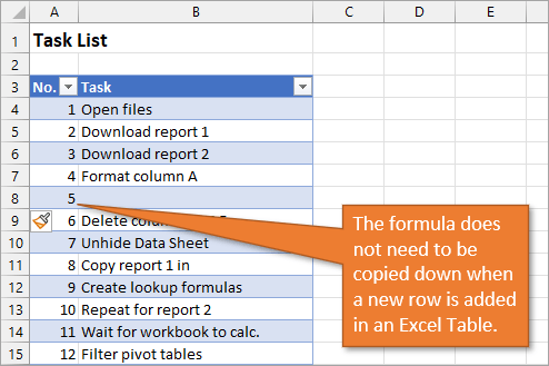
When we copy down the formula, we have a numbered list that will adjust when we add or delete rows. However, when adding a row, we will have to copy the formula into the newly inserted cell.
This additional step of copying the formula into new rows can be avoided if we use Excel Tables.
3. Create a Dynamic List Using a Formula in an Excel Table
If we write the same formula but we use an Excel table, the only difference we will make in the formula is that we reference the column header instead of the absolute cell value.
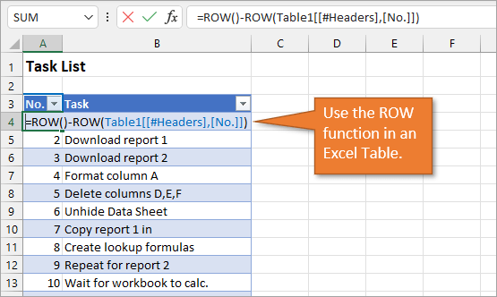
Because we are using an Excel Table, the formula automatically fills down to the other rows. When we add a row to the table, the formula will automatically populate in the new cell.
4. Create a Dynamic List Using Dynamic Array Formulas
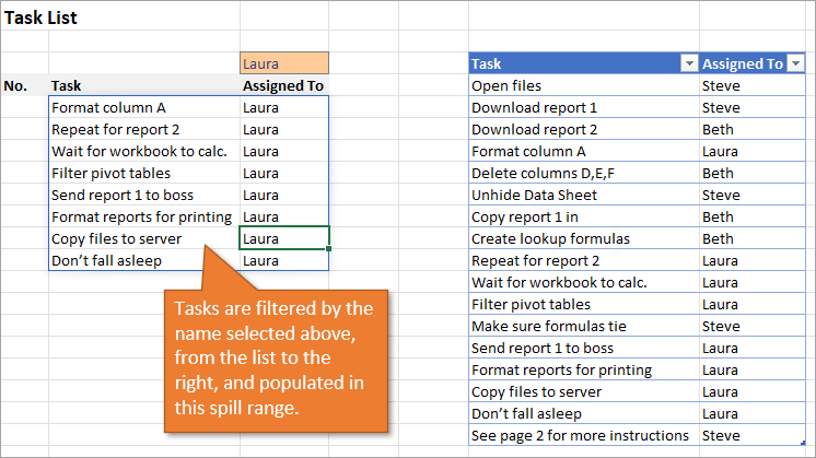
Below, I have a table that is populated using Dynamic Array Formulas. The FILTER formula spills a range of results based on whatever name is selected in the orange cell.
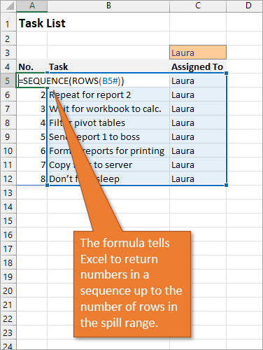
The Dynamic Array formula we will use is SEQUENCE. This will return a sequence for the number of rows we identify in the formula. To tell Excel how many rows there are, we will use the ROW function as the argument for sequence. The argument for ROW is just the spill range. The way to notate the spill range is to simply place a hashtag after the name of the first cell in the range. So our formula looks like this:
=SEQUENCE(ROWS(B5#))
Once we complete our formula and hit Enter, the list will be numbered.
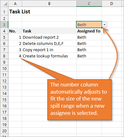
With this formula in place, if the size of the range changes when a new name is selected, the numbered column for the list will automatically adjust as well.
Bonus Tip: Formatting Your Numbered List
If you want to add periods or other punctuation to your numbered list:
- Select the entire list and right-click to choose Format Cells. Or use the keyboard shortcut Ctrl + 1.
- Choose the Custom option on the Number tab.
- Then in the Type field, type in the number 0 with whatever punctuation you would like to surround your number.
Here, I've just added a period.
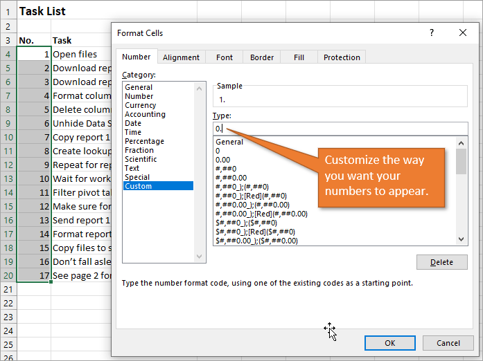
When you hit OK, you will have formatted the entire selection.
Related Posts
Here are a few similar posts that may interest you.
- Excel Tables Tutorial Video – Beginners Guide for Windows & Mac
- New Excel Features: Dynamic Array Formulas & Spill Ranges
- How to Prevent Excel from Freezing or Taking A Long Time when Deleting Rows
Conclusion
I hope these four ways to create ordered lists are helpful for you. If you have questions or feedback, I would love to hear them in the comments. Have a great week!


Hi Jon,
The way that I do it is as follows:-
Cell A4 shows 1
Cell A5 is a formula “=A4+1”, then copy this formula down
If you delete or add a row simply copy the formula down again
Peter
Great , Thanks
I use this formula for a list that auto updates.
I have a header row in column 1, my list numbers in column A and my data in column B. I put this formula in cell A2, and then copy it down.
=IF(SUBTOTAL(103,B2)=0,””,IF(B2″”,MAX($A$1:OFFSET(A2,-1,0))+1,””))
This will only show a number if there is something in the corresponding cell in column B. It starts at 1, but if I overtype any number at all in column A then it will use that number from then on. If a row is hidden then it doesn’t count that as a number at all. If I don’t want a number on a row I simply delete the formula and the list continues on the next row using the next number
Parts of it I’m sure I borrowed from informative sites just like this one, and I think I’ve tinkered with it a bit since then. So thought I’d post a comment and pass it on…
Great tips! I never realized how easy it could be to create numbered lists in Excel. The method using the Fill Handle is a game changer for my reports. Thanks for sharing!
Great tips! I especially love the method using the Fill Handle; it makes numbering so much quicker. Thanks for sharing!
Great tips! I never knew there were so many ways to create numbered lists in Excel. The method using the “ROW” function was particularly helpful for my projects. Thanks for sharing!
Great tips! I especially found the method using the Fill Handle very helpful. It’s amazing how such simple techniques can save so much time in organizing data. Thanks for sharing these!
Great tips! I particularly found the method using the ROW function super helpful for dynamic lists. Thanks for sharing these techniques, they will definitely improve my Excel productivity!