10 Excel Tricks That Will Save You HOURS

In this post I share 10 simple Excel tips that will help you navigate faster, clean data quickly, and build more usable spreadsheets.

Each tip is short and practical, and designed to help save you time with everyday Excel tasks.

Video Tutorial

Watch on YouTube & Subscribe to our Channel

Download the Example File

1. Navigation Tricks

Quick navigation matters. You can jump to the last used cell in a column or row without keyboard shortcuts. This is one of the most underrated Excel tips.

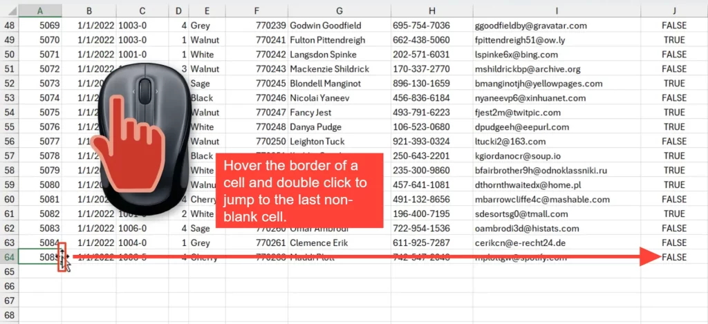
How it works:

1. Hover the mouse over a selected cell border until the cursor becomes a crosshair.
2. Double-click the bottom border to jump to the last used cell in the column.
3. Double-click the right border to jump to the last used cell in the row.

Want to select instead of just jump?

• Hold Shift and double-click the border to select the range from the active cell to the last used cell.

Note the caveat. If there are blank cells, the jump stops at the last non-blank cell before a blank. In that case, repeat double-click or use keyboard shortcuts like Ctrl+Down.

2. Clipboard Magic

This tip helps when you need to copy many ranges or items and paste them across sheets. It is one of the efficient Excel Time-Saving Tips And Hacks for repetitive copy and paste tasks.

Steps to enable and use:

1. Go to Home tab and open the Clipboard panel.
2. Click Options and enable “Collect Without Showing Office Clipboard”.
3. Copy multiple ranges or items. They appear in the Clipboard panel.
4. Switch to the destination sheet and click each item in the panel to paste it.

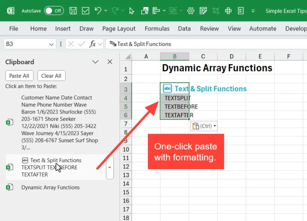
Benefits:

• No need to constantly switch between sheets.
• Maintains formatting when you paste directly from the panel.

Try this with dashboards or report assembly. It saves dozens of small clicks.

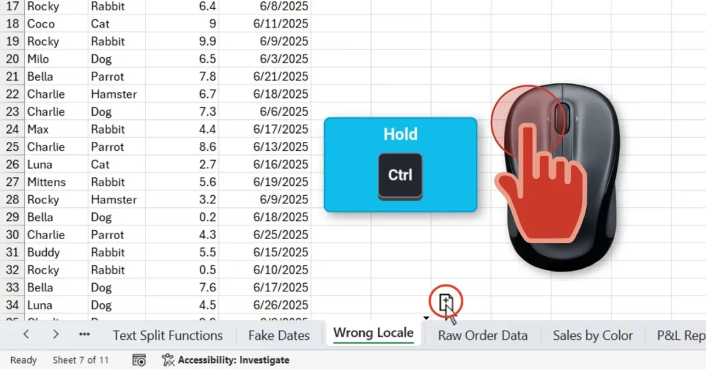
3. Convert Dates with Find & Replace

One classic cleanup task is converting dates stored as text into real date values. This trick is a quick Excel Time-Saving Tips And Hacks method that often works instantly.

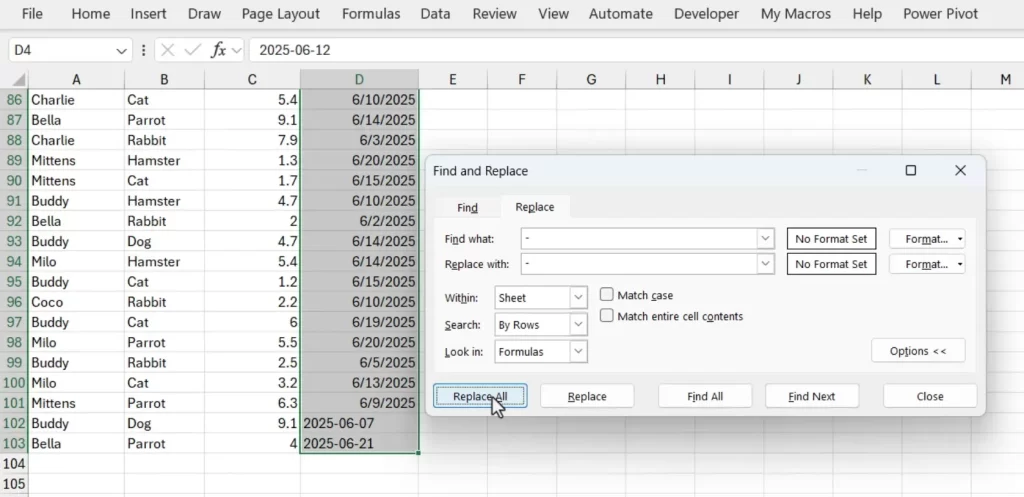
How to run it:

1. Select the column or range that contains the text dates.
2. Press Ctrl+H to open Find and Replace.
3. Enter the separator character in Find what and in Replace with. For example, type a dash in both fields.
4. Click Replace All. Excel reevaluates the cell content and converts recognisable strings into dates.

Important note. This works when the text dates already match your regional format. If dates are ambiguous or in a different format, use the next tip. Checkout our full-length tutorial on this find and replace technique for more details.

4. Fix Regional Date Formats With Text To Columns

In this example, the dates are in the Day-Month-Year format, but I am in the U.S., which has a default of Month-Day-Year format. The find and replace trick doesn't work in this scenario because there is a mismatch in the regional formats.

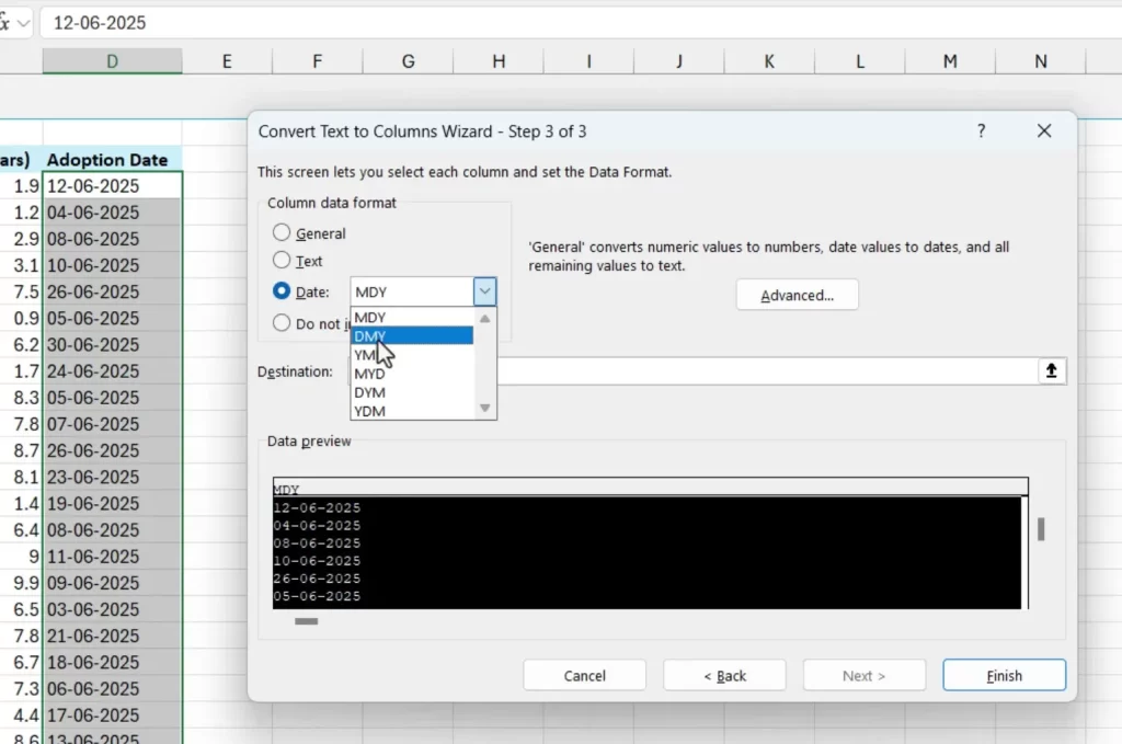
Therefore, we can use Text to Columns. 

Follow these steps:

1. Select the date column first.
2. Go to Data tab and choose Text to Columns.
3. In step one choose Delimited and click Next.
4. Click Next again in step two without changes.
5. In step three choose the actual format of the text dates. For example, choose DMY if your data is day-month-year.
6. Click Finish. Excel converts the text into proper date values that follow your regional settings.

Use this when dates show incorrect months or years after a simple replace. Text To Columns gives you control and predictable results. 

Here's an in-depth tutorial on using Text to Columns for fixing dates.

5. The Fastest Way to Duplicate A Sheet

Creating a copy of a sheet is common when building monthly reports. The drag+Ctrl method is one of those simple Excel hacks that will speed up your workflow.

How to duplicate:

1. Left click and hold the sheet tab you want to copy.
2. Drag it to the right or left where you want the copy.
3. Hold the Ctrl key. A small plus icon appears on the cursor.
4. Release the mouse button to create a duplicate sheet.

You can copy multiple selected sheets using the same technique. This beats the slower right-click Move Or Copy dialog.

6. Elegant Workbook Navigation

Want a dynamic table of contents with live thumbnails? Use Paste Special Linked Picture and hyperlink the picture to the sheet.

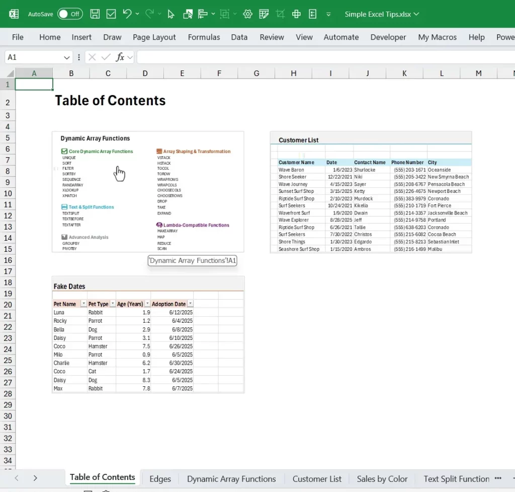
Steps:

1. Select the area you want to use as a thumbnail and press Ctrl+C to copy.
2. Go to your index sheet. Right-click and choose Paste Special, then choose Linked Picture.
3. Move and resize the image as needed.
4. Right-click the picture, choose Link, then Link To Place In This Document and pick the sheet to jump to.

Benefits:

• Thumbnails update automatically when the source sheet changes.
• Clickable images make navigation intuitive for users.

To polish the look, use Picture Format and Crop to match tile sizes. Add a border if you want a consistent design.

7. Quickly Add or Remove Borders

Borders from exports can clutter a report. Use keyboard shortcuts to remove or add borders fast. This is a practical member of the Excel Time-Saving Tips And Hacks list.

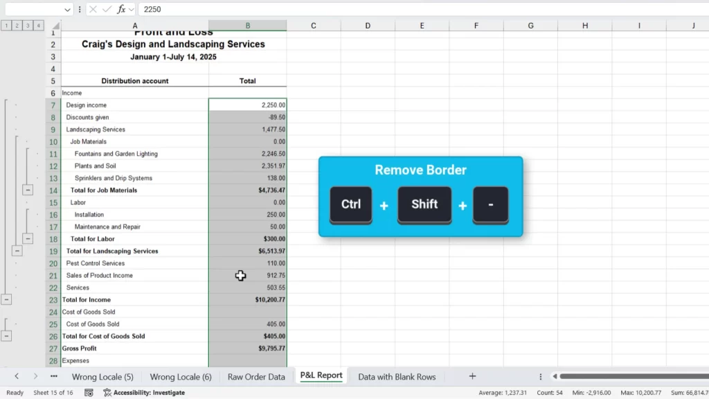
Shortcuts to remember:

1. Ctrl+Shift+- removes all borders in the selected range.
2. Ctrl+Shift+7 adds an outer border around the selected cells.

These shortcuts are fast and consistent. The dash key is usually between zero and equals on US keyboards.

8. Select Blank Cells to Flag Missing Data

Flagging missing data is an essential step in the data cleanup process to improve accuracy and eliminate errors.

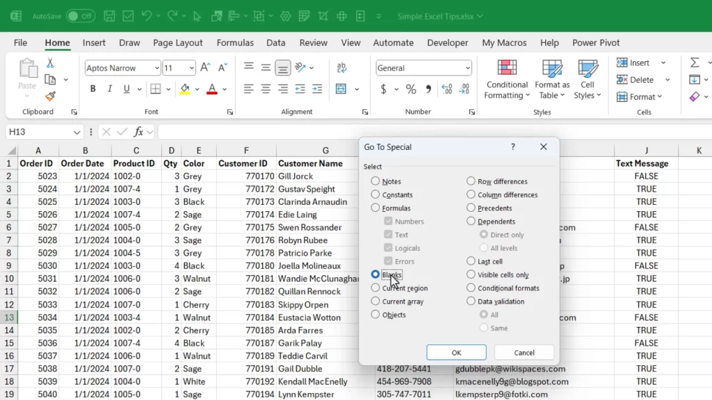
1. Press Ctrl+G or F5 to open Go To. Click Special.
2. Select Blanks and click OK. Excel highlights all blank cells in the active range.
3. Apply a fill color like yellow to indicate missing values.

The visual flag helps colleagues know exactly where data needs entry. It is a simple but effective communication method.

Here are some keyboard shortcuts for selecting entire columns with blank cells.

9. Insert Blank Rows

Often, times we need to add blank rows between existing rows so we can insert new data or do calculations.

The easiest way to do this is to:

1. Select multiple rows.
2. Right click the row headers and choose insert (keyboard shortcut: Ctrl++).
   The shortcut is hold the Ctrl key and press the plus key on the number pad. If you are on a laptop that doesn't have a numberpad, then press Ctrl+Shift+=

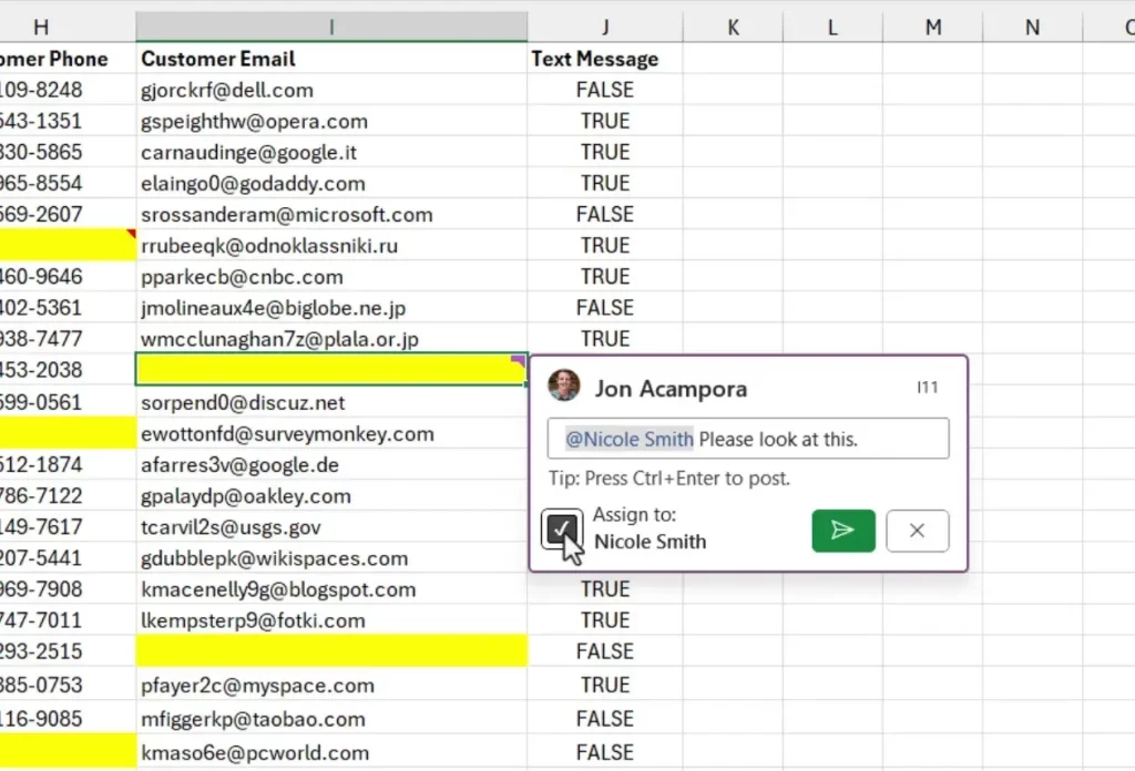
10. Adding Cell Notes or Comments

Inserting multiple rows and leaving notes for colleagues is another common task. Use selection and shortcuts to do it fast. 

Insert rows:

1. Select the number of rows you want to insert.
2. Right-click and choose Insert or press Ctrl+Plus.
3. Excel inserts that many blank rows above the selection.

Add notes or comments:

• Press Shift+F2 to add a note to the active cell.
• In Microsoft 365, press Ctrl+Shift+F2 to add a modern comment. You can @mention coworkers and assign tasks right from the comment.

Short notes speed handoffs. Modern comments improve collaboration in shared workbooks.

Final Thoughts

Learning these simple techniques will make you faster and more confident in Excel. And they will compound into huge time savings over the long term.

Try one tip per day and add it to your toolkit. When you combine these habits, you will build cleaner, faster, and more professional spreadsheets.

 If you want to learn about other tools in Excel like Power Query, macros, and VBA, then check out our free class called the Modern Excel Blueprint. You will learn the tools and techniques that are the most critical in the modern AI era. 

Register for the Free Excel Training Class