Bottom Line: Use the Find & Replace feature in Excel to quickly convert text to dates.
Skill Level: Beginner
Video Tutorial
Download the Excel File
You're welcome to use the same expense sheet that I've used as an example in the video. You can download it here:
Converting Text to Date Format
You might find that when you export data from online and financial programs such as QuickBooks Online, cells that are formatted as a date don't transfer over with the same format. They may look like dates, but they their data type is actually text.
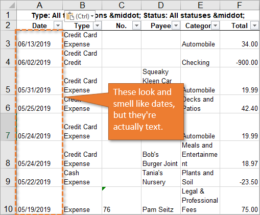
I'd like to show you a quick tip to quickly convert all of those text cells to dates.
How to Tell If Your Dates Are Actually Text
A couple of quick ways to tell if the data type for your cell is text or date include taking a look at either the number format drop-down menu or the filter drop-down menu.
Number Format Drop-Down
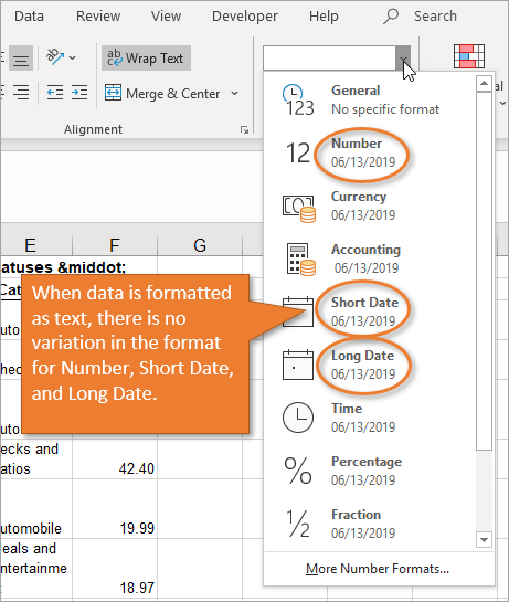
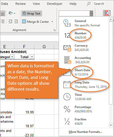
If you go to the Number Format drop-down menu on the Home tab, you will see how the formatting would look for each of the categories in the drop-down. When the data is text, you can see that the Number, Short Date, and Long Date options all look the same because Excel is not recognizing the data as a date.
If the cells were in date format, they would look like this instead:
Filter Drop-Down
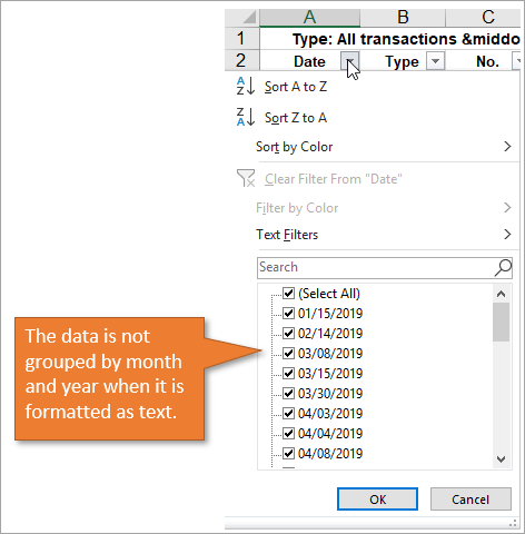
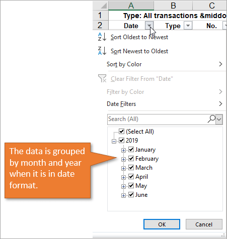
Another way to tell if a column of data is in text format is to look at the filter drop-down. If the entries aren't being grouped by Excel into months and years, Excel is not recognizing them as dates.
When formatted as dates, you can see the month and year groupings like this:
Use Find & Replace to Evaluate Cells
A quick and easy way for Excel to evaluate these cells and to recognize them as dates is to use the Find & Replace feature. On the Home tab of the Ribbon, click on the Find & Select menu and choose Replace….
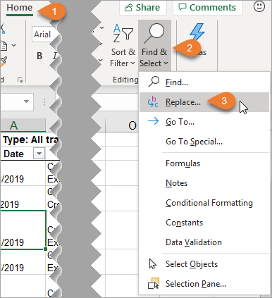
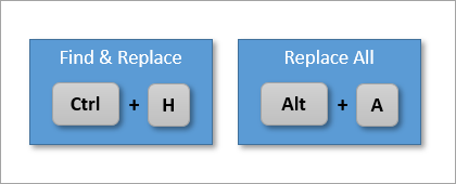
This brings up the Find and Replace window. (The keyboard shortcut to bring up this window is Ctrl + H.)
If your dates are formatted with forward slashes (/), you are going to enter a forward slash into BOTH the Find what and Replace with fields. If your dates are formatted with dashes (-), then use dashes.
Then click Replace All. (The keyboard shortcut for Replace All is Alt + A.)

By replacing these symbols, you are essentially forcing Excel to take a look at each of the cells you've selected, so that it can recognize their contents as dates.
Keyboard Shortcuts
Here are the keyboard shortcuts to open the Find & Replace Window and Replace All. Alt + i is the shortcut for Find All on the Find window, which is another one I use frequently.
What If My Default Date Format is Different?
The Find and Replace technique will NOT work if your regional date format is different from the date format that the data is in.
In this example the date uses the following format: mm/dd/yyyy
I am in the U.S. and this is the same as the regional date format we use. The regional date format is set in the operating system (Windows or MacOS), NOT in Excel.
If you are in a different country and your regional date format is dd/mm/yyyy or something different, then this technique will not work.
Workarounds
There are still many ways to convert the text to dates.
You can change the regional date settings in your operating system to match the date format in the data. I wouldn't recommend this unless you are only dealing with data from another country and constantly running into this issue.
Another option is to use Text to Columns or one of the other suggestions made in the comments section below. I will do a follow-up post on some of those solutions.
*A big thanks to Pieter, Simon, and Jonathan for pointing out this issue in the comments. We appreciate your support!
Bonus Tip
If you are exporting from an online or financial system, see if there is an option to export your data in a .CSV file. If so, it can help to avoid this problem of exporting dates as text.
Conclusion
So, if you find that your filter drop-down menu isn't grouping by month and year, or date specific formulas are not calculating correctly, you should check your data to make sure Excel is reading it as a date data type. If not, a quick run through the Find & Replace feature should set things straight.
What other ways would you go about fixing this problem? Please leave a comment below with suggestions on other techniques you would use.
Thank you! 🙂


Often times Excel does not recognize dates because of leading and trailing spaces. The solution is to run find and replace to remove all spaces. The trim function can also be used in a macro.
Great point! Thanks again Tim! 🙂
I use the following macro to remove excess spaces in date fields:
Sub TrimCells()
‘ Removes excess spaces from selected cells
Dim rng As Range, cell As Range
Set rng = Selection
For Each cell In rng
If IsEmpty(cell.Value) Then GoTo Skip
If Not cell.HasFormula And (cell.Value WorksheetFunction.Trim(cell.Value)) Then
cell.Value = WorksheetFunction.Trim(cell.Value)
End If
Skip:
Next cell
End Sub
Awesome! Thanks Tim! 🙂
Another way to ‘fix’ it is to put a 1 into an empty cell then copy it and select the date range and paste special with multiply selected. Format date as desired.
PC Keyboard Shortcuts:
Copy – ctrl+c
Select range – ctrl+shift+ arrow key in desired direction
Paste special/Multiply – alt+e+s+m
Format cells – ctrl+1
Sorry, I’m not familiar w/ribbon lettering and/or locations. I use keyboard shortcuts a lot and they tend to be pre-ribbon ones.
Thanks Tanya! I love keyboard shortcuts too! 🙂
I like to use Power Query. Make your data a table, and then Get Data, From Table (Excel 2016). Then once the query is opened, click on the column with the dates where the text icon is and change it to dates.
Thanks David! 🙂
Excellent tip Jon! Thank you!
Thanks Marci! 🙂
Hi Jon,
Thanks for the hints. If the grouping of dates in a pivot table doesn’t work, something’s wrong with the raw date. Which means you’re a step ahead obviously, but sometimes it happens, that I realize I need to get back, and change the “wannabe” dates to real dates.
Greg
Hi Greg,
Great point! I should have mentioned that this an essential step cleaning up data to work with pivot tables. Thanks! 🙂
My solution is to select the column, then go to data and select text to columns. I don’t alter anything at that point, I just select finish. Magically the text will become a date. this works as well or better for numbers stored as text. Rather than selecting a range and looking for the little hidden menu that pops up asking if I want to convert the text into numbers, and then waiting an eternity for it to actually process the entire range, this makes the change almost instantaneously.
Thanks Karl! 🙂
In a helper column one could use =date cell*1; or =DATEVALUE(Date Cell) – and copy paste by value over the range
or select range and select macro or hot button
Sub ConvertTextDateFormat()
Dim rng As Range
For Each rng In Selection
rng.Value = DateValue(rng)
Next rng
End Sub
Awesome! Thanks Jim! 🙂
We have the opposite problem: when excel is being too smart for its own good, and changes numbers that look like dates – but aren’t – into date formats.
We frequently pull data out of our inventory management system. Things like “10-49”, which signify a quantity range, are always changed by excel to Oct-49 (Oct 1st, 1949)! Changing the cell format to “text” or “general” then reverts the cell value to the date code ie. 18172. The actual text “10-49” is completely lost – you have to type ’10-49 into the cell to force excel to see the value as text. With a large data set, using find/replace works by searching the date (as long as you get the date format right!) and replacing-all with ‘text.
Often there’s just so many of them… 1-9 (1-Sep), 10-99 (Oct-99)… you get the picture. Interestingly things like 50-99 arent affected as excel cannot make a date from that.
Is there another way? Can the “auto-date” format be tamed?!!
Great question Jeremy! Yes, there are probably more than a few ways to go about it. One way is to use Power Query to import the data into Excel.
You can change the data type for each column before bringing it into Excel. In this case you would change that column to Text. Power Query will usually add a “Changed Type” step which automatically detects data types. You can either delete that step, or add an additional step to change the data type.
I’ll add this one to my list for future posts. I think it will make a great example of using Power Query.
Great workaround! I typically select the column, type Ctrl+1 to invoke the Format Cells dialog, click the Number tab, in the Category list box select Date, then click the OK button.
Thanks Jimmy! In this case the dates are stored as text, and changing the number format will NOT change the values to a date data type in Excel. We have to use another workaround like the Find and Replace trick or one of the other solutions mentioned in the comments here.
Wow Jon!
I didn’t know this trick!!! All these years I would copy a blank cell and paste special and use add operation. Thanks for sharing this tip.
Thanks Rudra! Happy to hear it helped and I appreciate you sharing the copy/paste trick. 🙂
Good post. I receive a monthly file with about 70K dates in a 20190702 layout, formatted as persistent text. I use:
=mid(A2,5,2)&”/”&right(A2,2)&”/”&left(A2,4)
Then use text-to-column (which is the only way I have figured out how to get the cells to quit reverting back to text), then copy and paste formula over the different columns needing conversion. Sounds lengthy, but really only takes a few minutes.
I recently had problems converting text to date because spaces weren’t spaces and hyphens weren’t hyphens.
That is to say, the spaces were “hard spaces”. They showed up when I copied the dates to Word.
A trick I often use to remove pesky “phantom” formatting is to copy the column to Notepad, then copy it back into a fresh column. That usually does the trick.
Thanks PG! 🙂
Great help, explains an issue I’ve been having with a pivot table. However, if your Excel is not set up to use the US date format, then those dates that don’t make sense as a date in, say, the UK date format will not be forced to format as dates. For example, 05/10/19 could be either 5th October 2019 (UK) or 10th May 2019 (US) so this is forced to reformat as a date. However, 04/14/19, or 14th April 2019 in US format, is not a recognisable date in UK format, 4th Fourteen-ember 2019!! Consequently a mix of cells, some reformatted as dates, some still as general, is the result. It is important also to check the source data is using the expected date format.
Good point Simon! I’m going to add a section to the post that explains more about this potential issue. Hopefully the data you are exporting will be in your local date format, in which case this technique would work, but I realize that’s not always the case. Thanks again! 🙂
The find/replace method does not work for me with your sample expenses file. Office365 Home.
The number formatting drop-down changes from General to Date, but they’re still not actually dates. All just text, no grouping and no difference between any of the previews.
I have to use this method:
Data | Text to Columns | Delimited | Uncheck all delimiter boxes | match the Date to suit (MDY in this case) | Finish
Hi Gary,
This could be the case if you are outside the U.S. and your local date format is something other than MM/DD/YYYY. I’ll add a section to the article with more info on this issue. Thanks! 🙂
Find & Replace doesn’t work in the sample file provided. I’m not sure why it would, since removing the slashes from “06/13/2019” merely results in “6132019”, which is still not a value that Excel can recognize as a date.
A better solution in this example is to simply use the VALUE function. So in the sample file provided, you would add the formula “=VALUE(A3)” to cell G3 and copy it down. This will convert the dates to “General” format, and then the whole column can be converted to any date format you like.
Hi PG,
It sounds like you didn’t add the slash character to the Replace With field. The slash needs to be in BOTH fields in the Find and Replace window. I hope that helps.
Copy any blank/empty cell. It must be a truly empty cell, not one that is pretending to be empty by using “” as its formula output. Then select the desired range of offending dates — even entire column(s) — and use Paste Special (Ctrl+Alt+V) with the Values and Add choices.
This will force Excel to do “math” (adding zero) to all of the values. And as you might know, when Excel attempts math on an otherwise text formatted value, a numeric conversion happens whenever the value is recognizable as a numeric (or date) format. Any cells that contain true text or anything else that can’t be converted to a number are left alone, and any blank cells remain blank — i.e. you won’t end up with a zero in all the cells that were previously blank.
The real beauty is that this will even work for text like Wednesday, July 3, 2019 or $5,372.18 or other recognizable date/number formats that might not be as easily handled by a find/replace trick.
Very cool! I like that the other cells that contain true text are not impacted.
Thanks for sharing this tip, David! 🙂
Select the cells you want to check and run this macro:
Sub Chg_Text_to_Date()
Dim cell As range
For Each cell In Selection
If IsDate(cell) Then
cell.Value = DateValue(Trim(cell.Value))
Selection.NumberFormat = “m/d/yyyy”
End If
Next
End Sub
Awesome! I love the VBA solution! Thanks Doug! 🙂
I get this problem very often.
This tip is very helpful, thank you!
Thanks Ana! 🙂
Another method I’ve only recently started using is Data / Text to Columns (under Data Tools). The intended use is to split text into columns, but it can also convert text dates into true dates. It’s also a good way to convert numeric text to true numbers more easily than what I used to do (Paste Special Multiply by 1).
Thanks for the suggestion Michael! Text to Columns seems to be a popular choice and I’ll do a follow-up on it. 🙂
Nice trick didn’t know till now 😀
when facing this kind of problem i use (Alt+A+E)…ENTER…Enter..Enter
most of the times works, without telling that format of date we want.
Thanks for sharing
Thanks for sharing the Text to Columns solution, Carlos! 🙂
Great trick, BUT, you need to ensure that the date format in the spreadsheet matches what is set in your preferences. In my case: Australia uses DD/MM/YYYY.
Good point Pieter! I’ll add a section to the post that explains this. Thanks!
Hi Jon
Thank you for this excellent trick.
To address the non-US date format, I used the following formula:
=(MID(A3,4,2)&”/”&LEFT(A3,2)&”/”&MID(A3,7,4))*1
And it helped!
Thanks once again.
Very usefull trick Jon. Text to column Alt+E+E+Enter 3 times also works for this. Thank you.
Thanks for sharing an alternate solution Hari! 🙂
Thank you for the new info
Many times I came to the problems of finding text data in the shape of date which gave me incorrect information when I linked such data to formulas e.g. countifs or when I used advanced filter.
In such cases I use different method which can be applicable with different dates writing like shown below.
Date
04‐07‐2019
05.07.2019
04‐07‐2019
07.07.2019
04‐07‐2019
09/07/2019
10‐07‐2019
If we want to change the text to dates by using replace method, we need to do it in 3 stages. 1 replace for each separator so that we can cover all the data.
There is another way to convert text dates to date format in one go which is by using “Text to Column” tool within Data tap. And I used this way many times.
First select the data
Then select “Text to Column” in Data tap
Then select NEXT
New window will appear then select NEXT again
Now select Date, but make sure to select the right format or date, month and year similar to the arrangement in the text.
Then select “Finish”
Next, open the filter and you can see the data became in date format and grouped accordingly
For better explanation, I prepared a blog in pdf format which downloadable following link below.
https://drive.google.com/file/d/1uqd8kVEsgCrMCgYvkdkpDj7gUanPhyUP/view
Thank
Maki S. Hussain, PMP
Baghdad, Iraq
Thanks so much Maki! Text to Columns is a great alternate solution, especially when your local date format is different from the source file OR you have different date formats in the column. I appreciate you creating the post with instructions. I’ll be doing a follow-up post & video with this technique.
Thanks again! 🙂
I am afraid to inform you that this trick is not working for all the cells instead it is working for few cells only. I mean i have selected all the cells i.e. A3 to A65 and did Cnrl+H…
But only few calls such as A3, A35 to A51, A55 to A59 & A62 are only getting chnaged as dates but others are not.
Kinldy look into it and revert.
Hi Ashish,
As Pieter mentioned in a comment below, this is likely due to your local date format being set to a different format. The example file contains dates in the MM/DD/YYYY format. The date and time format of your operating system would need to match this.
This is the default date format in the U.S. If you are in a different country where the default is DD/MM/YYYY then this trick will not work. You could use an alternate method like Text to Columns or Power Query.
However, the data you are exporting might be in your local format, and in that case the Find and Replace method would work. I’ll add a note about this to the article.
I hope that helps. Thanks again! 🙂
Jon: I don’t understand why the same technique does not work for non-US date formats. Surely Excel is just evaluating the input – as you indicated in your video – so what does it matter if the format is slightly different, so long as the input contains a forward slash?
Hi I Often ran in the same problem with exported data from a PLC logging. It is even worse because it is timestamped. Both date and timestamp are often in US regional mode depending on the manufacturer of the PLC, I’m using European style dd/mm/yy 13h45.
In the past i used techniques like TRIM LEFT RIGHT etc to get it right or start from the csv export and split it into columns.
However Power Query is really the most appropriate tool to do this conversion, especially if you press the “text symbol” (or date, decimal,…) left of the column name; it offers a wide range of conversions including the most brilliant one “using locale”… This choice is not in the top menu so be aware!
Using Power Query removes the need for VBA code, or repeating manual steps life FIND/REPLACE etc. Just drop a new file in the dedicated folder and it runs very smooth. I make these import methods for colleagues and they find it very user friendly!
Nice. My favourite method (to convert any number stored as text, including dates), is using paste special to multiply the cells by 1. Like this:
Type a number 1 (one) in any blank cell
Copy the cell with the 1 in it
Select the range if cells that should be numbers, but aren’t
Bring up the Paste Special dialog box (I use CTRL+ALT+v)
From the Paste Special dialog box, select Values and Multiply
🙂
I think this is easiest & most elegant solution. Thanks Danielle.
In reading through the comments, I see there are several ways to convert text dates to real dates, but many are multi-step approaches: A helper column with text manipulation formulas, cell helpers to multiply, VBA, or some other method. Yours is the cleanest solution I have seen and had not known about.
Thanks for the tip!
Excel also hates written-out days of the week — “Thursday, July 11, 2019” for example, will never be recognized as a date, even if it EXACTLY matches the “long version” of dates in the date styles. You first have to delete the day. Then it will recognize it.
I have to fix dates like that numerous times daily. So I have a macro that deletes all days of the week for my specified column.
Hi Jon
Thank you for this excellent trick.
To address the non-US date format, I used the following formula:
=(MID(A3,4,2)&”/”&LEFT(A3,2)&”/”&MID(A3,7,4))*1
And it helped!
Thanks once again.
The telco companies provide call logs with the date field using UTC or AEST to denote the date/time reference in the date field cell, across multiple time zones. This means i have to remove this to get excel to recognise it as a ‘date’ format. Be great to have a macro to adjust this to the local time zone and make it date/time format for other processing.
Hello,
Thanks for this method , it really helped.
Appreciate your work .
Keep Posting these type of ideas.
thanks Jon
great method
Have learned something thanks
Thanks for Helping us.
I have had this problem for as long as I have have had a computer. The way i have solved it never fails. I just skip the column where the date is supposed to be and put the date where the message is. Problem solved!
In this video “How to Convert Text to Dates with Find & Replace” is there any way that this problem can be fixed by some query or in BIP itself before exporting it??
Please respond to this.
Thank you
This was a very easy way to convert the text to date format. However I face a issue when my date is d/mm/yy. When I use find and replace to all cells, it converts text dates to date format for all date which are in dd/mm/yy and ignores the ones which are in d/mm/yy. How can I put 0 before d to get a dd format
Thanks in advance!
what happens if I have one preceding # and then dates two digits for month and two for year, but the preceding # that was provided I cannot remove it? I need the dates for expiration to be in this format mm/yy but cannot remove the # and does not take the format as text?
Excel is the most awesome piece of software – so flexible and powerful. However, Excel’s failure to implement ISO 8601 as the date format puzzles and annoys me. I have read ISO 8601-2004 and it says the date is written yyyy-mm-dd only. I tried to wake people up at the company I worked for but people do not want to change and keep writing stupid stuff like 4/2/07 !
There is no formula out there to convert TEXT date format 2022-Feb into an actual date. I have checked and cannot make any of the formulas you have work for this issues. There is nothing online either?
’09-03-2022 how to change this date format to 09-Mar-22. plz guide
a date field came out as a formula field “=DATE(2021,9,16)”
How do I convert this to a date?