How to Calculate Daily Averages with a Pivot Table

Bottom line: Learn how to calculate the average of a daily total amount across month, quarters, years, or even categories with a pivot table.

Skill level: Intermediate

Video Tutorial

Download the Excel File

You can download the Excel files below.  The BEFORE file just contains the source data, and can be used to follow along with the video.  The AFTER video contains the solution and sample pivot tables.

Average of Total Daily Sales

Kevin, a member of The Pivot Ready Course, asked a great question about calculating the average of total daily sales in a pivot table.

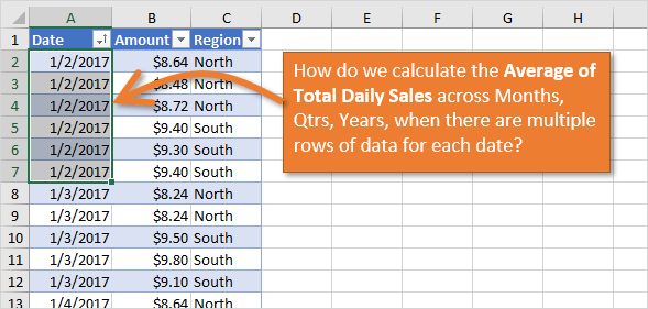
In this case his data set contained a sales transaction in each row.  There are multiple sales per day, so the dates will repeat in the Date column.

If we use the regular Average calcluation type in the pivot table, the result will be the average amount per transaction.  This is NOT what we want.

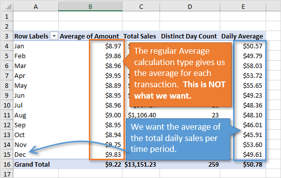
Instead, we want to see the average daily total across a larger time period like months quarters or years.

Why Analyze Daily Averages?

The daily average metric can be useful in comparing trends for daily totals across time period (months, quarters, etc.) or even categories (regions, departments, days of the week, etc.)

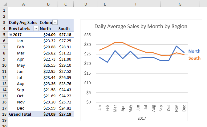
We can use a line chart or column chart to quickly see how the daily average changes over time.

How the Calculation Works

IMPORTANT NOTE: You will need Excel 2013 or later for Windows for this method.  This includes Office 365.  Unfortunately, this will not work on Excel 2010, or the Mac versions of Excel.

This technique uses DAX measures in the Power Pivot Data Model.   We are going to use the DISTINCTCOUNT function to calculate the unique number of days in the data set.  DISTINCTCOUNT is a DAX function in Power Pivot.

We then divide Total Sales by the Distinct Day Count to get the Average of Total Daily Sales.  This can be any amount (numeric value).  It does NOT have to be sales data.

[Average of Total Daily Sales] = [Total Sales]/[Distinct Day Count]

Here are the steps to creating the pivot table and measures.

Step 1: Insert a Pivot Table & Add to Data Model

The first step is to insert a pivot table from your data set.

Important: Click the “Add this data to the Data Model” checkbox on the Create PivotTable Window.

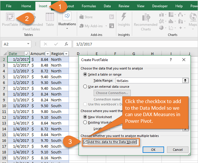
This will add the data to Power Pivot and allow us to write DAX measures for the Distinct Count calculation.

Step 2: Create the DAX Measures

Next we need to create the measures.  We are going to create explicit measures for three calculations:

1. Total Sales = SUM([Amount])
2. Distinct Day Count = DISTINCTCOUNT([Date])
3. Daily Average = [Total Sales]/[Distinct Day Count]

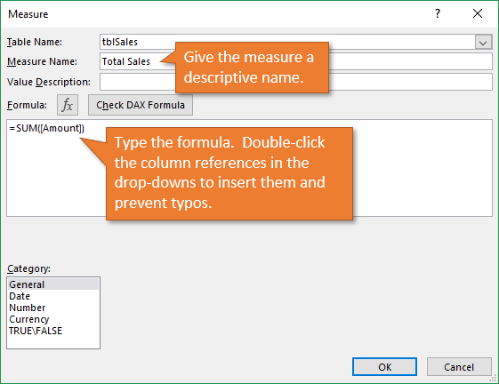
To create a measure:

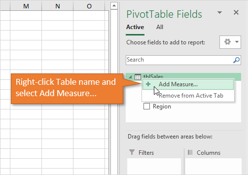
1. Right-click the Table name in the Pivot Table Fields List.
   
2. Select Add Measure.  The Measure Window will appear
3. In the Measure Name box type: Total Sales
4. In the Formula box type: =SUM([Amount])
   
5. Click OK.

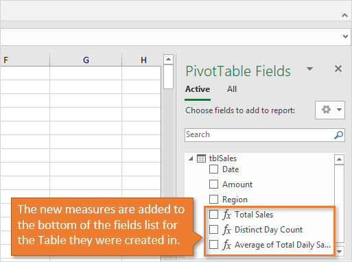
The measure will be created and added to the bottom of the Fields List.  Repeat the steps above for the other two measures.

Implicit vs Explicit Measures

For the first two formulas we could also create the calculations by dragging the Amount and Date fields into the Values area, then changing the calculation type as need.  These are know as implicit measures when we use Excel to create the measure by dragging and dropping fields.

The other option is to write the formulas in the Measure window, like we did above.  These are known as explicit measures because we clearly explained or defined them in the formula editor.

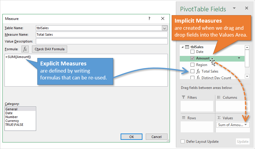
One advantage of the explicit measures is that we can continue to use them in other formulas or pivot tables.  Now that we have defined the Total Sales measure, it will be available in all new pivot tables from the data model.

We can also re-use the Total Sales measure, as we did in the Daily Average measure, and continue to build more complex formulas with it.  This saves time and makes formula writing more efficient in the long run.

There are also advantages when using Power BI and bringing the data model back into Excel.  My friend Avi shows an example in this video where Implicit measures are not imported to Excel from Power BI.

Step 3: Add the Measures to the Pivot Table

The next step is to add the measure fields to the Values area of the pivot table.

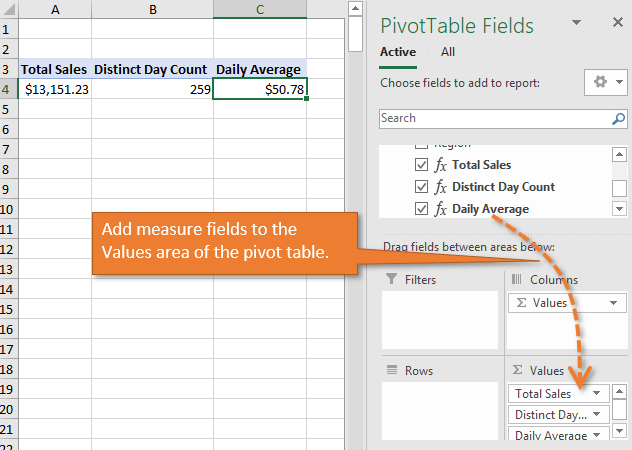
You do NOT need to add all of the measure fields to the pivot table.  The calculations will still work even if you only add the Daily Average field to the Values area.

However, the Total Sales and Distinct Day Count fields can be a nice addition to the pivot table.  They might help show additional trends or explain why a daily average is high/low for a specific period.

The same measures will also work in Power BI, since Power BI uses Power Pivot to create relationships and measures.  Checkout my course on Dashboards & Data with Power BI to learn more.

Step 4: Create Date or Category Groupings

We now need to add fields to the Rows and/or Columns Areas to create the trend report.

For this example, we will add the Date field to the Rows area and Group it by Year, Quarter, and Month.

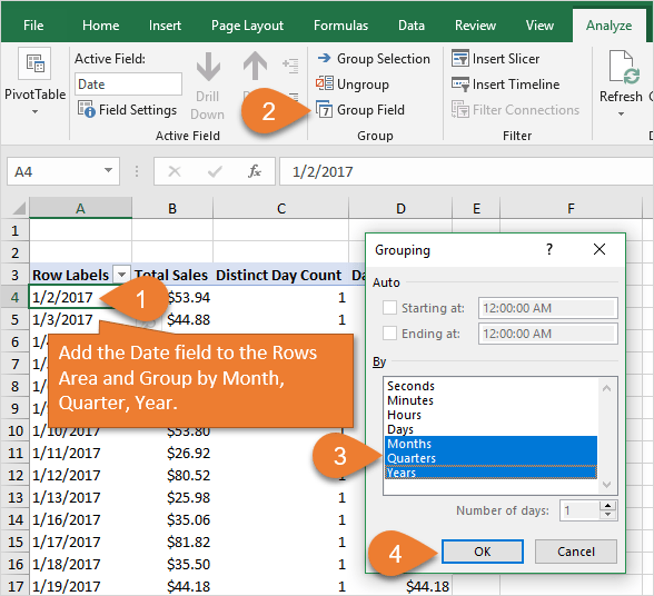
Checkout my article on Grouping Dates in a Pivot Table VERSUS Grouping Dates in the Source Data to learn more about date grouping.

I also have an article on The Calendar Table (Date Dimension) Explained for Power Pivot & Power BI.  Calendar tables allow us to create relationships between different data sources.  They can also be used if your company is on a fiscal calendar.

Make Sure Subtotals are Turned On

If you don't see numbers for the Year, Quarter, or Month lines, then the Subtotals are turned off in your pivot table.  Here is a screenshot that shows how to turn the subtotals on.

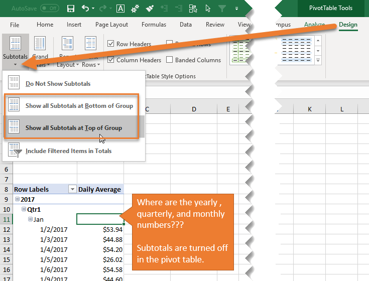
To turn the Subtotals on in a pivot table:

1. Select a cell inside the pivot table.
2. Select the Design tab in the ribbon.
3. On the Subtotals drop-down menu, select “Show all Subtotals at Bottom of Group” or “Show all Subtotals at Bottom of Group”.
4. You should now see the subtotal calculations for the row area groupings (year, quarter, month).

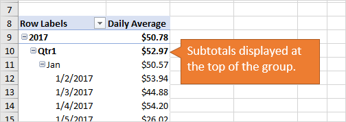
Step 5: Analyze the Trends

Finally we can add a quick pivot chart to analyze the trends of the daily averages.  Here is a line chart that compares the Average Daily Sales by Month and Region.

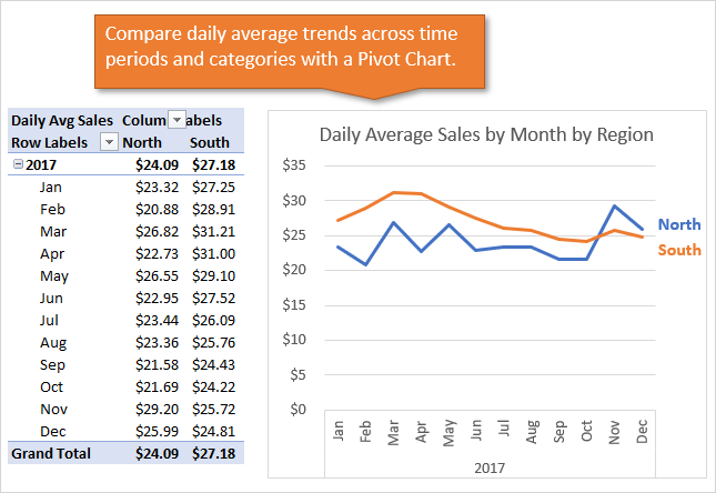
We can see that the North region did better than the South in the last two months of the year.  And the South had a declining trend after March.

What Do You Use Daily Averages For?

So, that is one way to calculate daily averages with pivot tables using Power Pivot and DAX Measures.  DAX measures are amazingly powerful, and this simple example only scratches the surface of their capabilities.

I'd love to know what you use daily average metrics for.  Please leave a comment below and let us know.  Thanks so much! 🙂

Free Training Webinar on the Power Tools

If you are currently using pivot tables, but feel like you aren't getting the most out of them, then I have a free training just for you.

Right now I'm running a free training webinar on all of the Power Tools in Excel. This includes Power Query, Power Pivot, Power BI, pivot tables, macros & VBA, and more.

It's called The Modern Excel Blueprint. During the webinar I explain what these tools are and how they can fit into your workflow.

You will also learn how to become the Excel Hero of your organization, that go-to gal or guy that everyone relies on for Excel help and fun projects.

The webinar is running at multiple days and times. Please click the link below to get registered and save your seat.

Click Here to Register for the Free Webinar