The Ultimate Guide to Excel Filters with VBA Macros – AutoFilter Method

Bottom line: Learn how to create macros that apply filters to ranges and Tables with the AutoFilter method in VBA.  The post contains links to examples for filtering different data types including text, numbers, dates, colors, and icons.

Skill level: Intermediate

Download the File

The Excel file that contains the code can be downloaded below.  This file contains code for filtering different data types and filter types.

Writing Macros for Filters in Excel

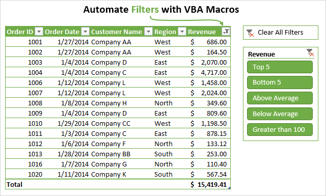
Filters are a great tool for analyzing data in Excel.  For most analysts and frequent Excel users, filters are a part of our daily lives.  We use the filter drop-down menus to apply filters to individual columns in a data set.  This helps us tie out numbers with reports and do investigative work on our data.

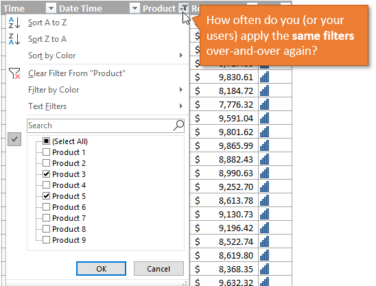
Filtering can also be a time consuming process.  Especially when we are applying filters to multiple columns on large worksheets, or filtering data to then copy/paste it to other worksheets or workbooks.

This article explains how to create macros to automate the filtering process.  This is an extensive guide on the AutoFilter method in VBA.

I also have articles with examples for different filters and data types including: blanks, text, numbers, dates, colors & icons, and clearing filters.

The Macro Recorder is Your Friend (& Enemy)

We can easily get the VBA code for filters by turning on the macro recorder, then applying one or more filters to a range/Table.

Here are the steps to create a filter macro with the macro recorder:

1. Turn the macro recorder on:
   1. Developer tab > Record Macro.
   2. Give the macro a name, choose where you want the code saved, and press OK.
2. Apply one or more filters using the filter drop-down menus.
3. Stop the recorder.
4. Open the VB Editor (Developer tab > Visual Basic) to view the code.

If you've already used the macro recorder for this process, then you know how useful it can be.  Especially as our filter criteria gets more complex.

The code will look something like the following.

Sub Filters_Macro_Recorder()
'
' Filters_Macro_Recorder Macro
'

'
    ActiveSheet.ListObjects("tblData").Range.AutoFilter Field:=4, Criteria1:= _
        "Product 2"
    ActiveSheet.ListObjects("tblData").Range.AutoFilter Field:=4
    ActiveSheet.ListObjects("tblData").Range.AutoFilter Field:=5, Criteria1:= _
        ">=500", Operator:=xlAnd, Criteria2:="<=1000"
End Sub

We can see that each line uses the AutoFilter method to apply the filter to the column.  It also contains information about the criteria for the filter.

This is where it can get complex, confusing, and frustrating.  It can be difficult to understand what the code means when trying to modify it for a different data set or scenario.  So let's take a look at how the AutoFilter method works.

The AutoFilter Method Explained

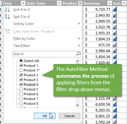
The AutoFilter method is used to clear and apply filters to a single column in a range or Table in VBA.  It automates the process of applying filters through the filter drop-down menus, and does all that work for us. 🙂

It can be used to apply filters to multiple columns by writing multiple lines of code, one for each column.  We can also use AutoFilter to apply multiple filter criteria to a single column, just like you would in the filter drop-down menu by selecting multiple check boxes or specifying a date range.

Writing AutoFilter Code

Here are step-by-step instructions for writing a line of code for AutoFilter

Step 1 : Referencing the Range or Table

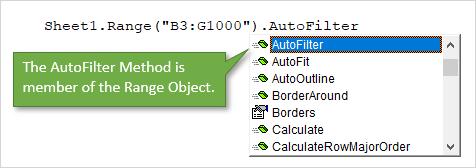
The AutoFilter method is a member of the Range object.  So we must reference a range or Table that the filters are applied to on the sheet.  This will be the entire range that the filters are applied to.

The following examples will enable/disable filters on range B3:G1000 on the AutoFilter Guide sheet.

Sub AutoFilter_Range()
'AutoFilter is a member of the Range object
  
  'Reference the entire range that the filters are applied to
  'AutoFilter turns filters on/off when no parameters are specified.
  Sheet1.Range("B3:G1000").AutoFilter
  
  'Fully qualified reference starting at Workbook level
  ThisWorkbook.Worksheets("AutoFilter Guide").Range("B3:G1000").AutoFilter

End Sub

Here is an example using Excel Tables.

Sub AutoFilter_Table()
'AutoFilters on Tables work the same way.

Dim lo As ListObject 'Excel Table

  'Set the ListObject (Table) variable
  Set lo = Sheet1.ListObjects(1)
  
  'AutoFilter is member of Range object
  'The parent of the Range object is the List Object
  lo.Range.AutoFilter
  
End Sub

The AutoFilter method has 5 optional parameters, which we'll look at next.  If we don't specify any of the parameters, like the examples above, then the AutoFilter method will turn the filters on/off for the referenced range.  It is toggle.  If the filters are on they will be turned off, and vice-versa.

Ranges or Tables?

Filters work the same on both regular ranges and Excel Tables.

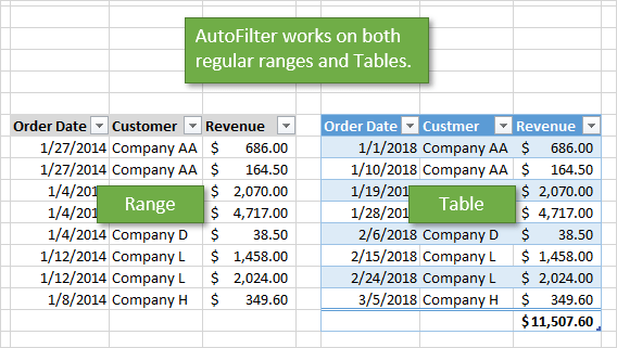
My preferred method is to use Tables because we don't have to worry about changing range references as the table grows or shrinks.  However, the code will be the same for both objects.  The rest of the code examples use Excel tables, but you can easily modify this for regular ranges.

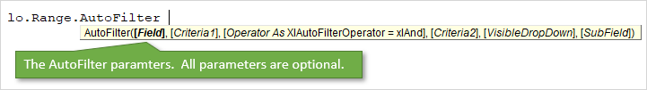
The 5 (or 6) AutoFilter Paramaters

The AutoFilter method has 5 (or 6) optional parameters that are used to specify the filter criteria for a column.  Here is a list of the parameters.

Name	Req/Opt	Description
Field	Optional	The number of the column within the filter range that the filter will be applied to. This is the column number within the filter range, NOT the column number of the worksheet.
Criteria1	Optional	A string wrapped in quotation marks that is used to specify the filter criteria.  Comparison operators can be included for less than or greater than filters.  Many rules apply depending on the data type of the column.  See examples below.
Operator	Optional	Specifies the type of filter for different data types and criteria by using one of the XlAutoFilterOperator constants.  See this MSDN help page for a detailed list, and list in macro examples below.
Criteria2	Optional	Used in combination with the Operator parameter and Criteria1 to create filters for multiple criteria or ranges.  Also used for specific date filters for multiple items.
VisibleDropDown	Optional	Displays or hides the filter drop-down button for an individual column (field).
Subfield	Optional	Not sure yet…

We can use a combination of these parameters to apply various filter criteria for different data types.  The first four are the most important, so let's take a look at how to apply those.

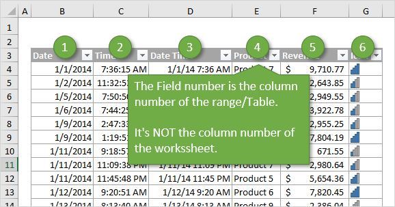
Step 2: The Field Parameter

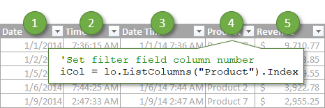
The first parameter is the Field.  For the Field parameter we specify a number that is the column number that the filter will be applied to.  This is the column number within the filter range that is the parent of the AutoFilter method.  It is NOT number of the column on the worksheet.

In the example below Field 4 is the Product column because it is the 4th column in the filter range/Table.

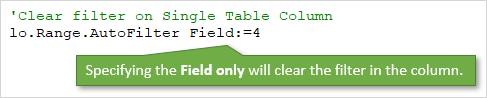
The column filter is cleared when we only specify the the Field parameter, and no other criteria.

We can also use a variable for the Field parameter and set it dynamically.  I explain that in more detail below.

Step 3: The Criteria Parameters

There are two parameters that can be used to specify the filter Criteria, Criteria1 and Criteria2.  We use a combination of these parameters and the Operator parameter for different types of filters.  This is where things get tricky, so let's start with a simple example.

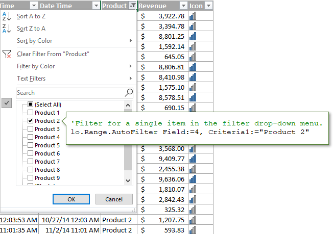
'Filter the Product column for a single item
lo.Range.AutoFilter Field:=4, Criteria1:="Product 2"

This would be the same as selecting a single item from the checkbox list in the filter drop-down menu.

General Rules for Criteria1 and Criteria2

The values we specify for Criteria1 and Criteria2 can get tricky.  Here are some general guidelines for how to reference the Criteria parameter values.

• The criteria value is a string wrapped in quotation marks.  There are a few exceptions where the criteria is a constant for date time period and above/below average.
• When specifying filters for single numbers or dates, the number formatting must match the number formatting that is applied in the range/table.
• The comparison operator for greater/less than is also included inside the quotation marks, before the number.
• Quotation marks are also used for filters for  blanks “=” and non-blanks “<>”.

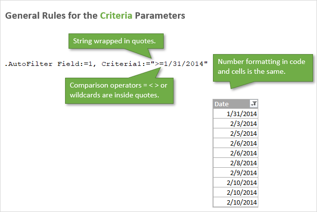
'Filter for date greater than or equal to Jan 1 2015
lo.Range.AutoFilter Field:=1, Criteria1:=">=1/1/2015"

' The comparison operator >= is inside the quotation marks
' for the Criteria1 parameter.

' The date formatting in the code matches the formatting
' applied to the cells in the worksheet.

Step 4: The Operator Parameter

What if we want to select multiple items from the filter drop-down?  Or do a filter for a range of dates or numbers?

For this we need the Operator.  The Operator parameter is used to specify what type of filter we want to apply.  This can vary based on the type of data in the column.  One of the following 11 constants must be used for the Operator.

Name	Value	Description
xlAnd	1	Include both Criteria1 and Criteria2.  Can be used for date or number ranges.
xlBottom10Items	4	Lowest-valued items displayed (number of items specified in Criteria1).
xlBottom10Percent	6	Lowest-valued items displayed (percentage specified in Criteria1).
xlFilterCellColor	8	Fill Color of the cell
xlFilterDynamic	11	Dynamic filter used for Above/Below Average and Date Periods
xlFilterFontColor	9	Color of the font in the cell
xlFilterIcon	10	Filter icon created by conditional formatting
xlFilterValues	7	Used for filters with multiple criteria specified with an Array function.
xlOr	2	Include either Criteria1 or Criteria2. Can be used for date and number ranges.
xlTop10Items	3	Highest-valued items displayed (number of items specified in Criteria1).
xlTop10Percent	5	Highest-valued items displayed (percentage specified in Criteria1).

Here is a link to the MSDN help page that contains the list of constants for XlAutoFilterOperator Enumeration.

The operator is used in combination with Criteria1 and/or Criteria2, depending on the data type and filter type.  Here are a few examples.

'Filter for list of multiple items, Operator is xlFilterValues
lo.Range.AutoFilter _
          Field:=iCol, _
          Criteria1:=Array("Product 4", "Product 5", "Product 6"), _
          Operator:=xlFilterValues

'Filter for Date Range (between dates), Operator is xlAnd
lo.Range.AutoFilter _
          Field:=iCol, _
          Criteria1:=">=1/1/2014", _
          Operator:=xlAnd, _
          Criteria2:="<=12/31/2015"

So that is the basics of writing a line of code for the AutoFilter method.  It gets more complex with different data types.  So I've provided many examples below that contain most of the combinations of Criteria and Operator for different types of filters.

AutoFilter is NOT Additive

When an AutoFilter line of code is run, it first clears any filters applied to that column (Field), then applies the filter criteria that is specified in the line of code.

This means it is NOT additive.  The following 2 lines will NOT create a filter for Product 1 and Product 2.  After the macro is run, the Product column will only be filtered for Product 2.

'AutoFilter is NOT addititive.  It first any filters applied
'in the column before applying the new filter
lo.Range.AutoFilter Field:=4, Criteria1:="Product 3"
  
'This line of code will filter the column for Product 2 only
'The filter for Product 3 above will be cleared when this line runs.
lo.Range.AutoFilter Field:=4, Criteria1:="Product 2"

If you want to apply a filter with multiple criteria to a single column, then you can specify that with the Criteria and Operator parameters.

How to Set the Field Number Dynamically

If we add/delete/move columns in the filter range, then the field number for a filtered column might change.  Therefore, I try to avoid hard-coding a number for the Field parameter whenever possible.

We can use a variable instead and use some code to find the column number by it's name.  Here are two examples for regular ranges and Tables.

Sub Dynamic_Field_Number()
'Techniques to find and set the Field based on the column name.
  
Dim lo As ListObject
Dim iCol As Long
  
  'Set reference to the first Table on the sheet
  Set lo = Sheet1.ListObjects(1)
  
  'Set filter field
  iCol = lo.ListColumns("Product").Index
  
  'Use Match function for regular ranges
  'iCol = WorksheetFunction.Match("Product", Sheet1.Range("B3:G3"), 0)

  'Use the variable for the Field parameter value
  lo.Range.AutoFilter Field:=iCol, Criteria1:="Product 3"

End Sub

The column number will be found every time we run the macro.  We don't have to worry about changing the field number when the column moves.  This saves time and prevents errors (win-win)! 🙂

Use Excel Tables with Filters

There are a lot of advantages to using Excel Tables, especially with the AutoFilter method.  Here are a few of the major reasons I prefer Tables.

• We don't have to redefine the range in VBA as the data range changes size (rows/columns are added/deleted).  The entire Table is referenced with the ListObject object.
• It's easy to reference the data in the Table after filters are applied.  We can use the DataBodyRange property to reference visible rows to copy/paste, format, modify values, etc.
• We can have multiple Tables on the same sheet, and therefore multiple filter ranges.  With regular ranges we can only have one filtered range per sheet.
• The code to clear all filters on a Table is easier to write.

Filters & Data Types

The filter drop-down menu options change based on what type of data is in the column.   We have different filters for text, numbers, dates, and colors.  This creates A LOT of different combinations of Operators and Criteria for each type of filter.

I created separate posts for each of these filter types.  The posts contain explanations and VBA code examples.

• How to Clear Filters with VBA
• How to Filter for Blank & Non-Blank Cells
• How to Filter for Text with VBA
• How to Filter for Numbers with VBA
• How to Filter for Dates with VBA
• How to Filter for Colors & Icons with VBA

The file in the downloads section above contains all of these code samples in one place.  You can add it to your Personal Macro Workbook and use the macros in your projects.

Why is the AutoFilter Method so Complex?

This post was inspired by a question from Chris, a member of The VBA Pro Course.  The combinations of Criteria and Operators can be confusing and complex.  Why is this?

Well, filters have evolved over the years.  We saw a lot of new filter types introduced in Excel 2010, and the feature is continuing to be improved.  However, the parameters of the AutoFilter method haven't changed.  This is great for compatibility with older versions, but also means the new filter types are being worked into the existing parameters.

Most of the filter code makes sense, but can be tricky to figure out at first.  Fortunately we have the macro recorder to help with that.

I hope you can use this post and Excel file as a guide to writing macros for filters.  Automating filters can save us and our users a ton of time, especially when using these techniques in a larger data automation project.

Please leave a comment below with any questions or suggestions.  Thank you! 🙂