Bottom Line: Learn some Excel keyboard timesavers that will make you popular around the office.
Skill Level: Beginner
Uncommon But Useful
If you're not already considered a hero around at work, sharing these simple Excel shortcuts might help to elevate your status in the eyes of your coworkers. 🙂 These tips are not as well known as Ctrl + C for copy and Ctrl + V for paste, but they're almost just as useful.
1. Open an Options Menu
Win: Alt + ↓
Mac: Opt + ↓
This shortcut can be used in several different situations. For example:
- If your filters are turned on, you can open the filter drop-down menu from any of the headers.
- For cells with data validation lists, this shortcut will open the drop-down menu that displays your options.
- For cells that don't have data validation lists, this shortcut will bring up an auto-fill list containing all of the unique entries from the column that the cell is on.
- When writing formulas, you can see the argument options by placing your cursor over the relevant data and using the shortcut to see what other options are available for selection.
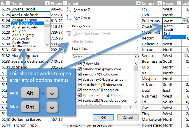
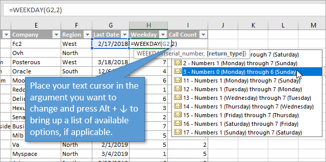
I've got more tips when it comes to filtering drop-down menus in this helpful article: 7 Keyboard Shortcuts for the Filter Drop Down Menus
2. Repeat Your Last Action
Win: F4 or Ctrl+Y
Mac: Cmd + Y
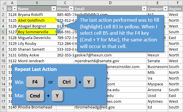
After performing an action on a cell in your worksheet, using this shortcut allows you to repeat the action in another cell. This includes applying number formatting, changing fonts and fill colors, inserting shapes, and more.
3. Select All Used Cells in a Column
Win and Mac: Ctrl + Shift + ↓
This is especially helpful if you have a spreadsheet with really long columns of data. If you want to select the entire column, just start at the top and use Ctrl + Shift + ↓ to highlight all the way to the end of the column.
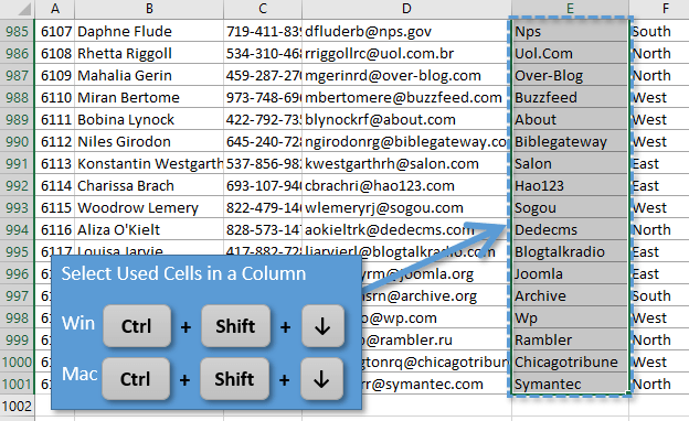
Now, if there are cells with no data in your column, this shortcut only selects the cells down to that first non-blank cell, so keep that in mind. Check out these tutorials for workarounds to that issue:
- 2 Keyboard Shortcuts to Select a Column with Blank Cells
- 7 Keyboard Shortcuts for Selecting Cells and Ranges in Excel
- 5 Keyboard Shortcuts for Rows and Columns in Excel
4. Copy a Sheet
Win: Ctrl + drag
Mac: Opt + drag
You can make a duplicate of an existing sheet using this shortcut.
- Start by clicking on the tab you want to copy.
- Then drag to the right until the down triangle arrow moves from the left of the tab to the right.
- Before releasing your click, hit the Ctrl button (Opt button for Macs) and you will see a little plus symbol (+) appear in the icon.
- When you release mouse button, the duplicate tab will appear to the right of the original.
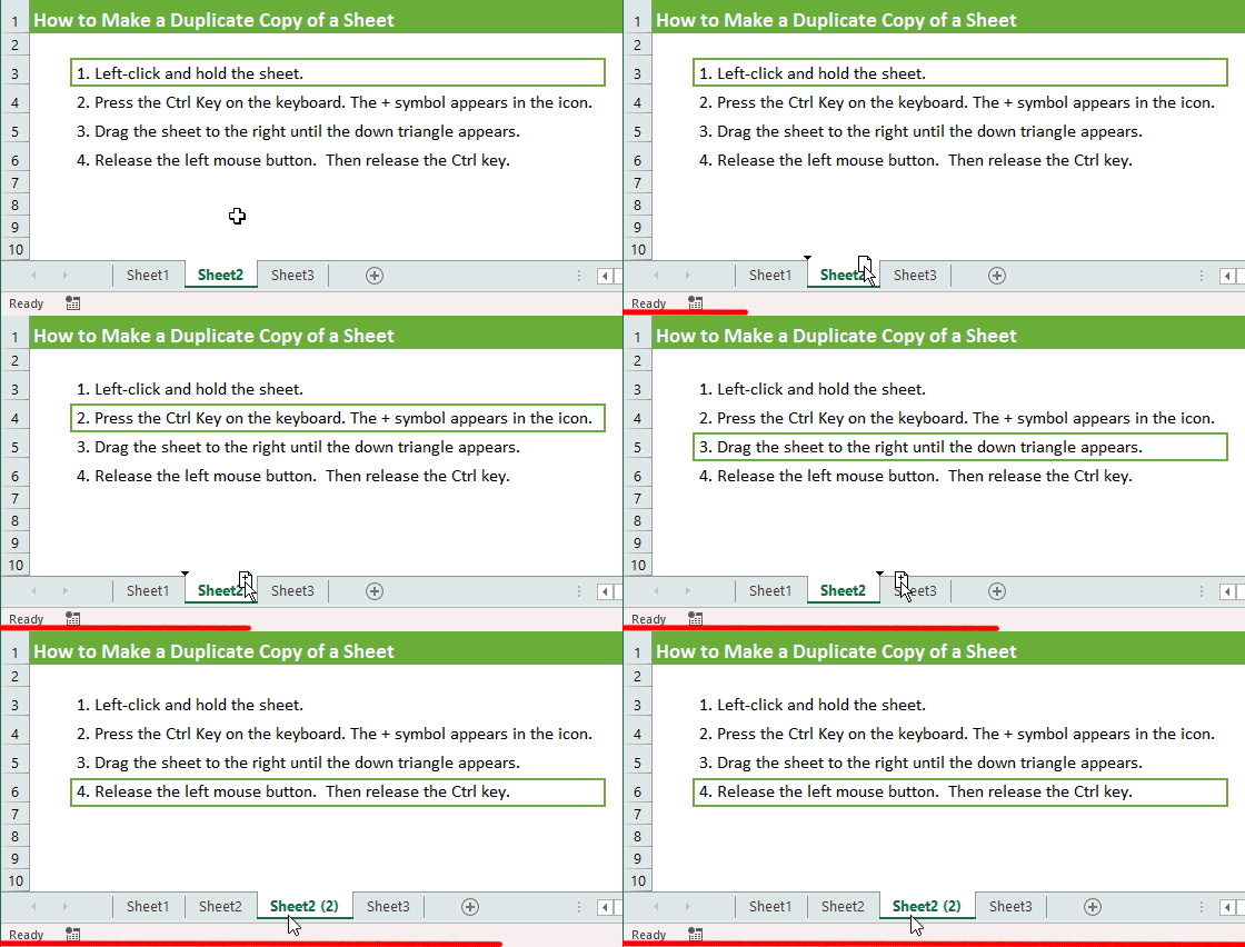
This procedure can also be done to copy multiple tabs at once.
Want some more tips and timesavers for working with tabs? Check out this post: 7 Shortcuts for Working with Worksheet Tabs in Excel
5. Toggling Between Sheets
Win: Ctrl + PgUp | Ctrl + PgDn
Mac: Fn + Cmd + ↑ | Fn + Cmd + ↓
Using this shortcut will move you to other open sheets in the workbook. The up shortcut will move you to the next tab to the right, and the down shortcut moves you to the left.
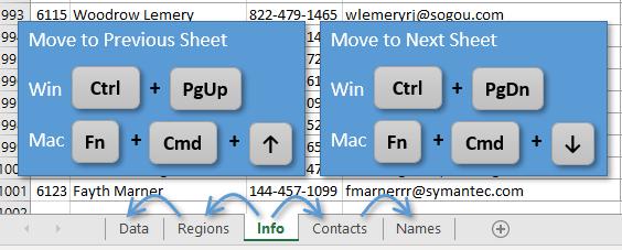
Some keyboards may not have the PgUp and PgDn buttons, so be aware of that. I have this article on the Best Keyboards for Excel Keyboard Shortcuts that you might want to check out.
6. Enter Today's Date and/or Time
For date:
Win and Mac: Ctrl + ;
For time:
Win: Ctrl + Shift + ;
Mac: Opt + ;
If you want to put the current date or time in a cell, use this shortcut. It will automatically enter the date or time from your computer system.
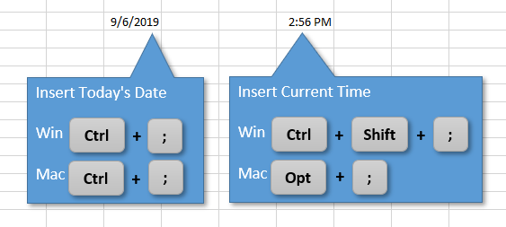
If you want both the date and the time in the same cell, just enter a space between the respective shortcuts.
(If you've entered the time in the cell, but it is not showing when you leave the cell, you may want to check the cell's format settings. You will probably have to change the format to an option that displays the time.)
Check out my article on how dates work in Excel for more details.
7. Sum a Range of Numbers (AutoSum)
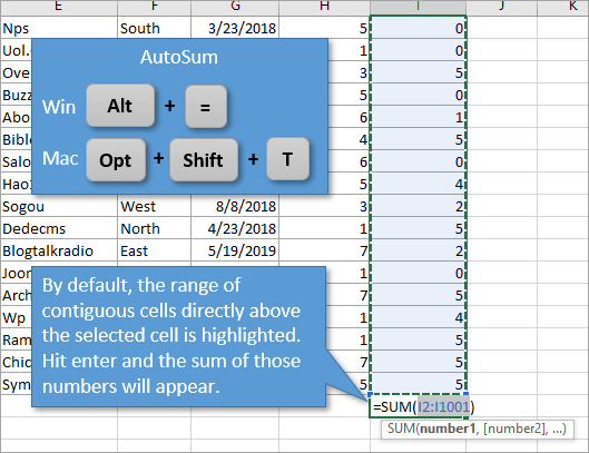
Win: Alt + =
Mac: Opt + Shift + T
If you want to quickly add all of the numbers in the range directly above a cell, just use this shortcut. The formula to add up the numbers is created automatically, and you can simply hit Enter to get your sum.
Conclusion
Have you used any or all of these shortcuts before? Can you see yourself putting some of them to use to save time and help others?
These 7 techniques are just the tip of the iceberg when it comes to all of the ways you can save time with keyboard shortcuts in Excel. What are some of your favorite and most-used shortcuts? Let me know in the comments below.


In shortcut 3, the END Key also works (instead of CTRL). However, if a cell contains a formula that evaluates to a BLANK it is also selected. Do you know if it there is a shortcut that will treat the formula as a BLANK?
Thanks Rich! Interesting, I never knew that about the End key instead of Ctrl. It’s kind of weird combination, but I found you can press and release End before pressing Shift+Down Arrow. Cool!
I don’t know of a shortcut that treats a formula returning a blank as an actual blank cell. You could potentially use the Find Window (Ctrl+F) to find the blank. Change the Look In option to Values. And change Search to by Columns if you are looking down a column.
I hope that helps. Thanks again and have a nice day! 🙂
Jon,
Thanks, I’ll be sharing this with my co-workers. But for some reason Tip #1 isn’t working for me. Maybe I changed some Option? The Ctrl +Alt + Down Arrow works when I have a Table. Any ideas why Alt + Down Arrow isn’t working with Data Filters?
Brian
Hi Brian,
I’m not exactly sure why Alt+Down Arrow wouldn’t be working. Do you have the cell in the header row selected? That’s the cell with the filter button in it.
And thanks for sharing the post. I appreciate your support! 🙂
Jon,
I have some code in my PMW that assigns Alt + Down Arrow to a macro. X (
This was awsome
Thanks Anton! 🙂
You picked a great bunch of shortcuts – I use them all!
Here are some more of my go-to time-savers:
1) Ctrl+Space … select entire column
2) Shft + Space … select entire row
3) Ctrl + +/- … insert/delete entire row/column (or cells if row/column not selected)
4) Ctrl + ‘ … repeat contents of cell above
5) Ctrl + r … repeat contents of cell to the left
6) Ctrl + 1 … format cells
And a couple that I just discovered:
1) Ctrl + 2 (or 3 or 4) … font bold (or italic or underline)
2) Ctrl + ( … hide row
3) Ctrl + ) … hide column
Are there also shortcuts for unhide row/column?
Thanks for keeping it fun!
Thanks Dave! Your list is awesome and I’ll add some of those to the next post on shortcuts.
Here is a post that explains the shortcuts to unhide rows/columns. It’s #4 in that post.
The shortcuts are Ctrl+Shift+( for rows and Ctrl+Shift+) for columns. However, the columns shortcut doesn’t always work and I explain a workaround on that post.
I hope that helps. Thanks again and have a nice day! 🙂
Copy Sheet just became my new best friend!!!! Thank you for sharing this!
I have a spreadsheet for payroll. Each sheet is a month and not only does it figure the payroll based on the time checked in and out but it carries forward YTD info and tracks vacation time used and balance. Each month I copy and paste for the next month and I have to reformat the page and change my YTD calculations for the current prior month (I hope I’m making sense here). I have a complete year now, so with this shortcut I can now copy the full year. Formatting copies along with the correct YTD formulas and all I have to do is empty the check-in/out fields – unless you are willing to share a macro that will do that for me 😉 .
The Current Time shortcut will also be useful here.
Question – I have protected and locked the sheet for co-workers so they can only enter times checking in and out. If I unprotect to copy for the next year, will it copy the locked cells so all I have to do is protect the sheet again?
Thanks again!
Hi Lori,
Awesome! I’m happy to hear it. I think the Copy Sheet shortcut is one of my favorites too because of how much time it saves. Going through the right-click menu is 4 to 5 clicks.
Your monthly process could definitely be automated with a macro. Since you are a member of our VBA Pro Course, you might want to submit this as a question for a VIP session. We have one coming up.
In regards to protected sheets and locked cells, YES, those properties and settings will be carried over to the new (copied) sheet. If the sheet is protected, then the new sheet will be protected as well.
I hope that helps. Thanks! 🙂
Alt-Enter in a cell to create a hard break. Shared it with my co-worker and made his day last week!
That’s a good one! I’ll add it to the list for future posts. Thanks! 🙂
This is one of my favorites!!
Thank you so much! I had been looking for a date and time shortcut 🙂
Awesome! Thanks Donna! 🙂
Wow! I have used Excel for 25 years. I consider myself to be an expert. I only knew about three of these “uncommon” shortcuts. Thanks. Always appreciate your knowledge and your well-done videos!
Thank you, Allen! I appreciate your support and honest reply. We will never run out of things to learn with Excel. I think that’s what makes it fun and challenging. 🙂
Oops! Sorry for the typo in your name. I corrected it. 🙂
Thanks for the shortcuts!
This is known, please give some more short cuts
You shared a shortcut within the past ~18ish months that has been a life saver but did not make your current list – copy and paste visible cells only using
Alt+; Ctrl+c Ctrl+v
In earlier versions I could use Find & Select to produce those results but I’ve been unable to make that work consistently in the past couple of versions.
I like your method much better anyway; a lot less work.
Thanks for all you do!
Awe yes, that’s one of my favorites too. Thanks for sharing it here, Mary! 🙂
Here is the link to the post on copy & paste visible cells only, for anyone that is interested.
It us really amazing. I have never used any of them before. Thank you.
Musa
Thanks Musa! 🙂
Always find something new to learn and appreciate the effort you put into these Youtube videos and emails.
My “go to” channel when l need to find something about Excel, explained in a logical informative manner.
To enter the same value, or formula, in a series of continuous cells, vertically or horizontally, select the entire range where you want the entry made, then type the value or formula into the first cell (the anchor cell) then press Ctrl + Enter. Either the same value, numeric or text, or the same formula with cell references adjusted as if you did drag and drop, will be entered into the entire range pre-selected.
yea…I get the new one
Ctrl + ;
and
alt =
Thanks
Thank you for this video, I love these shortcuts!
CTRL+SHIFT+L is my all time favourite shortcut. Use it so much!!
It turns column filters on or off.
thanks for you hint. I enjoy practicing them
Awesome stuff, John. As always, thank you for passing on your skillz to us. ( I spell it with a (z) lol.
One question though, was wondering when I use shortcut (Ctrl + =) it gives me subtotal formula. I’m using a PC.
Thank you so much! I have a question, I knew we can do ctrl shift + down to select all contents in the column but what if I want to select everything and then deselect one or more rows? e.g. if there is a row showing total number, I wouldn’t want to include that one. Not sure if it is possible? Thank you!
Excellent as ever Jon,.
Ctrl D to copy down
Ctrl R to copy right
both get used quite a bit & copy just the adjoining cell or if you select a few cells – including the one you want to copy – it fills them all.
Interesting. For me they only work if one highlights where to copy to AND if the copied cell is part of that highlighted range. Both work 1-D, but also 2-D, if I highlight a rectangle. Actually, now I don’t need to copy first, just highligh a cell. Curious.
Very weirdly, BOTH “Clear Contents” or take the action pressing the Delete key makes if I select an isolated cell (empty cells around it), and press either one.
Ahh… if Ctrl-R, it looks to the cell to the selected cell’s left and copies IT to the range or single cell. So if that’s blank, it copies/fills blanks, looking like Clear Contents. Same with Ctrl-D, just looking above.
Interesting. Wonder about formulas… Yep, just like copy and paste would act, changing references and all.
Trick to Select non-contiguous cells in a column.
1. select the whole columns by clicking the column letter
2. shift the active cell to the first cell (Ctrl+period)
3. Crtl+Shift+up arrow will select a bottom-up direction, so all the cells will be selected.
done
I find I need to press Ctrl-. twice. Once to reach the last cell in the column, once more to activate the top cell instead. Then do #3. Interesting though, did not know about Ctrl-. at all. Works equivalently in rows, but still needs done twice.
Further experimentation got me noticing that when I click a whole column, the active cell is ALWAYS the row 1 cell in the column. Then just “END-UP ARROW” brings the bottom of my selection from row 1,048,576 up to the last used cell in the column.
So select the whole column, then type “End-UP Arrow” to have all used cells in the column selected (all cells from row 1 down to the last row in the column with an entry).
Since the selection stays the row 1 cell, I can expand the selection downward from that point with “Shift-DOWN Arrow” if, for example, I might wish to include one more cell and put a “SUM()” in it with “Alt-=”.
Great Job
There are some errors….
Nr.7: WIN
Correct is: ALT + Shift + =
Nr.6: WIN
Correct is: CTRL + :
For #6, Alt-= works for me and Alt-Shift-= does nothing. For #7, bear in mind the “Shift-;” portion IS “:” so Ctrl-Shift-; and Ctrl-: are the same thing. But:
Ctrl-;
Ctrl-Shift-;
carries the relationship of the shortcuts more obviously. Like pairings of Ctrl-something making a copy and Ctrl-Shift-something moving the original (file, cell, whatever). You see the relationship and can reliably apply the idea to other things that could come in pairs. I think that’s why people express them this way.
With further use of Alt-=, I find that if one uses it with no values in any of the cells, Excel gives “SUM()” with nothing in the “()”. Not too useful as one then has to type a range anyway. But with some value anywhere in the range, it works as advertised.
Value though, not just content. If no numeric entry is in the range, you get the “()”. If you have letters AND numbers, it ignores the letters. It actually ignores them to the extent that any non-numeric cells that occur before the first numeric cell are cut out of the range. So if A1 has “a” and A2 has 6, using the range A1:A5 with the SUM going into A5 cuts the range it covers to A2 through A4.
So, no using it during setups, but once you have data, sure. I guess in setups, to have the accuracy of the programming setting the range, one could put a number in the top cell, do this to the range, then delete the inserted number. Typing sooner or later leads to typos so…
Hi Jon!
I love these shortcuts! Thanks for sharing!
This might not be relevant but I am curious of the gif under #4? May I ask how did you create that?
Jane
Experimenting for some of the ones in the article I came across a couple things, one pretty odd: Ctrl-9
If I do it with a range selected, H1:H23 perhaps, it does something like freezing panes, except when you freeze panes, you can still see anything visible at the moment you froze them, AND you can arrow or mouse into the non-moving region/s.
With this, the view shifts to row 24 being the top row visible and you cannot arrow or mouse up into it. So it’s like freezing the region above row 24 (no left side freeze) but rather different as well.
Further weirdness comes from the fact that if I select a cell in the next row (25 here), and do it again, that row also becomes non-viewable. BUT, if I leave at least one row alone and move down, to say, row 30, and do it, the row simply “Hides” (“Hide Row”). If I select a range in the viewable area, say rows 26 to 34, but leaving at least one row of the viewable area above them untouched, doing it again simply hides those rows. But if I include the first viewable row, the unviewable area moves down to include all so far.
(By the way, “Ctrl-0” works similarly with columns. Include the first viewable column in any range of cells and press it and those columns are all unviewable. But “Ctrl-Shift-0” does not revert it which is very odd.
Not sure how to revert it either. “Ctrl-Shift-9” (“Ctrl-(“) works on the absolute last one I’ve done, but repeated uses do not undo the other uses of it. A formal UNDO (“Ctrl-Z”) certainly does the trick though.
The region is unviewable, but not inaccessible. GoTo will take you to any cell inside it and you can make changes that you can verify by going to a viewable spot and entering, say, “=H14” to see your change to H14.
Maybe useful as a way to make some area completely unviewable? Not if there is a shortcut or command to revert it I guess, but otherwise… Though using GoTo to go to A1 and then moving about while watching the Formula Editor would reveal contents anyway. Unless they were made unviewable in the normal way. Hmm…
The other was that “Ctrl-Shift-<" ("Ctrl-<") seems to do what DELETE does. Might be useful someday if my Delete key doesn't work or some evil spreadsheet maker uses VBA to kill normal Delete-ing. Bet they don't know about this one! (If they do use VBA to kill Delete-ing AND put some of the spreadsheet's necessary logic into VBA, then opening without VBA would let one Delete, but also give one useless material as VBA won't be able to contribute to the processing. Since they'd never think of this shortcut, I'd win! You know, haven't run into that combination of factors in 34 years of spreadsheeting, but maybe someday… and I'd win!)
100
31 45 66
45 64 1
1 97 64
100
=RAND()*$A$1 =RAND()*$A$1
=RAND()*$A$1 =RAND()*$A$1
=RAND()*$A$1 =RAND()*$A$1
Hi Roy
I have a number of tables of data used for testing. This one runs from A3 to J22 and it has a Box & Whisker graph alongside the data.
If I select a row e.g. A12:J12 and then select Ctrl-0 the columns disappear and the data is not viewable by the graph either, There’s just an empty bordered space. I tried loads of key combinations to try to reverse it but with no success apart from finding one combination that completely locks the sheet, even the Undo arrow fails to work and I had to use Task Manager to close it. (System Interrupts showed 100% CPU usage) Doh!
I do not encounter the 100% system usage. I am able to revert the disappeared columns with Undo in the completely normal Undo manner (if I did more things, they get Undone before the columns re-appear). And I do see the chart contents disappearing as well.
The chart disappearing seems very strange, but I’m betting it’s not but rather is diagnostic. When I look for a way to treat the “gone” columns as simply Hidden, the usual commands, in, say, the Context Menu, are simply not there. Even when I do the same columns you did, and select column K back to the little box to the left of the column headers and above the row numbers. (That’s the usual way to select before being able to unhide leftmost columns that are Hidden.) Just… not there.
But, if I enter the Ribbon Menu, Home submenu, then the Cells subsubmenu, and select the Format subsubsubmenu from that, then go down that menu to the Hide and Unhide subsubsubsubmenu and then select Unhide Columns, BANG, they are back.
So it IS a way of Hiding rows or columns, as thought, but in a way that seems to disable some of the ways of undoing the hiding. For the rows, “Ctrl-9” hid them in the strange way, and “Ctrl-Shift-(” unhid them. Well, one act of hiding anyway. But for the columns, while “Ctrl-0” does hide them, “Ctrl-Shift-)” does not seem to ever unhide them.
The reason I said the Chart disappearing might be diagnostic is that a chart’s properties have the ability to deal with Hidden and Empty Cells, though what ability I do not know as for this experiment, columns visible or not, that feature was grayed out for me and I never use charts so I do not have experience with it from past use. But the fact of the button suggests one can make the chart ignore OR use either hidden OR empty cells in its data ranges.
In this case, seeing that button spoke to me saying the chart’s display went away because it was by default set to ignore data coming from hidden columns, and that since it was empty, it might very well be doing just that. That would mean the columns were hidden by the command and if I exhausted ALL ways to unhide them that I could find, I might find one way that was still available to me. I was even ready to open my spreadsheet with useful VBA Immediate Window commands to try getting the Immediate Window to unhide them.
If it ran the command but the columns did not re-appear, I would have gone back to thinking it was some odd new thing. But if it did unhide them, I would have thought it was just a… unique… way of hiding things that in some circumstances had unusual features.
Didn’t have to get to that point though as I found the commands in the Ribbon sub-sub-sub-sub-menu to be available rather than missing altogether or grayed out. And the unhide command worked, so clearly the problem was in fact that they were hidden.
Now I wonder how to access the grayed out “Hidden and Empty Cells” button in the Chart’s “Select Data Source” dialog box…
And I still wonder why this method of hiding rows and columns is so different in its aftereffects from other ways of hiding them.
It’s very exciting to know this marvelous shortcut keys. I’l be following you page, Sir.
Wow Jon, This has instantly transformed the work of my colleague and me. So grateful
Thanks, Jon. A couple of new ones for me here. Some others I really like are: CTRL + [ to jump to the cell(s) being reference in formulas on other sheets and CTRL + T to insert a table.
In the section #5 Tab Shift are your directions reversed? On my computer Ctrl pageup selects the tab to the left; Ctrl Pagedown selects the tab to the right. Just curious if it is my computer.
I love your helpful hints. Keep up your amazing work.
Just found a new key combo that applies to the finding the last cell used in a column. Never run into it before, and it acts differently depending upon what cell you have as your working cell when you use it.
Ctrl-| (“Control-Pipe”) or as some would prefer Ctrl-Shift-| or even Ctrl-Shift-.
First, select a column with Ctrl-Space Bar. Use Tab to NOT have the row 1 cell selected.
Then press Ctrl-Pipe. All the used cells (anything not a true blank, so =”” in a cell would see that cell selected) will be selected.
In addition, your working cell is now the row 1 cell. Pressing Shift-Tab “rolls you around” to the last used cell (like going off-screen at the top in a video game of yore and coming right up at the bottom as you do).
Done.
By the way, this selecting all the used cells thing works row-wise as well. In that case, the analogous “what cell is NOT your working cell” is the column A cell.
Be particular about that as the key combo works noticeably differently when the first row/column cell is the working cell when you press Ctrl-Pipe and so is not helpful for the “last cell” finding.
Aargh… Somehow I lost a backslash at the beginning: Ctrl-Shift- was the combo I meant to type, not Ctrl-Shift and a period to end the sentence…
These are great Jon! For #3 (Ctrl+Shift+Down Arrow), I have the same annoyance with blank cells in the column/row so I made two macros called Select To Bottom and Select To Right that highlight to the very end, including blanks!