How to Split Text in Cells Using Formulas

Bottom Line: Learn how to use formulas and functions in Excel to split full names into columns of first and last names.

Skill Level: Intermediate

Watch the Tutorial

Download the Excel Files

You can download both the before and after files below. The before file is so you can follow along, and the after file includes all of the formulas already written.

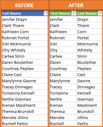
Splitting Text Into Separate Columns

We've been talking about various ways to take the text that is in one column and divide it into two. Specifically, we've been looking at the common example of taking a Full Name column and splitting it into First Name and Last Name.

The first solution we looked at used Power Query and you can view that tutorial here: How to Split Cells and Text in Excel with Power Query. Then we explored how to use the Text to Columns feature that's built into Excel: Split Cells with Text to Columns in Excel. Today, I want to show you how to accomplish the same thing with formulas.

Using 4 Functions to Build our Formulas

To split our Full Name column into First and Last using formulas, we need to use four different functions. We'll be using SEARCH and LEFT to pull out the first name. Then we'll use LEN and RIGHT to pull out the last name.

The SEARCH Function

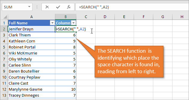
They key to breaking up the first names from the last names is for Excel to identify what all of the full names have in common. That common factor is the space character that separates the two names. To help our formula identify everything to the left of that space character as the first name, we need to use the SEARCH function.

The SEARCH function returns the number of the character at which a specific character or text string is found, reading left to right. In other words, what number is the space character in the line of characters that make up a full name? In my name, Jon Acampora, the space character is the 4th character (after J, o, and n), so the SEARCH function returns the number 4.

There are three arguments for SEARCH.

• The first argument for the SEARCH function is find_text. The text we want to find in our entries is the space character. So, for find_text, we enter ” “, being sure to include the quotation marks.
• The second argument is within_text. This is the text we are searching in for the space character. That would be the cell that has the full name. In our example, the first cell that has a full name is A2. Since we are working with Excel Tables, the formula will copy down and change to B2, C2, etc., for each respective row.
• The third and last argument is [start_num]. This argument is for cases where you want to ignore a certain number of characters in the text before beginning your search. In our case, we want to search the entire text, beginning with the very first character, so we do not need to define this argument.

All together, our formula reads: =SEARCH(” “,A2)

I started with the SEARCH function because it will be used as one of the arguments for the next function we're going to look at. That is the LEFT function,

The LEFT Function

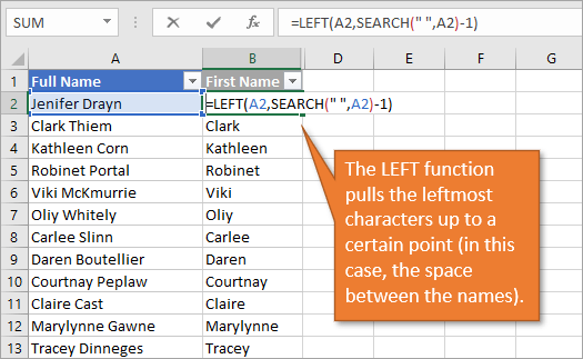
The LEFT function returns the specified number of characters from the start of a text string. To specify that number, we will use the value we just identified with the SEARCH function. The LEFT function will pull out the letters from the left of the Full Name column.

The LEFT function has two arguments.

• The first argument is text. That is just the cell that the function is pulling from—in our case A2.
• The second argument is [num_chars]. This is the number of characters that the function should pull. For this argument, we will use the formula we created above and subtract 1 from it, because we don't want to actually include the space character in our results. So for our example, this argument would be SEARCH(” “,A2)-1

All together, our formula reads =LEFT(A2,SEARCH(” “,A2)-1)

Now that we've extracted the first name using the LEFT function, you can guess how we're going to use the RIGHT function. It will pull out the last name. But before we go there, let me explain one of the components that we will need for that formula. That is the LEN function.

The LEN Function

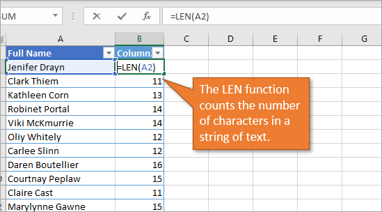
LEN stands for LENGTH. This function returns the number of characters in a text string. In my name, there are 12 characters: 3 for Jon, 8 for Acampora, and 1 for the space in between.

There is only one argument for LEN, and that is to identify which text to count characters from. For our example, we again are using A2 for the Full Name. Our formula is simply =LEN(A2)

The RIGHT Function

The RIGHT formula returns the specified number of characters from the end of a text string. RIGHT has two arguments.

• The first argument is text. This is the text that it is looking through in order to return the right characters. Just as with the LEFT function above, we are looking at cell A2.
• The second argument is [num_chars]. For this argument we want to subtract the number of characters that we identified using the SEARCH function from the total number of characters that we identified with the LEN function. That will give us the number of characters in the last name.

Our formula, all together, is =RIGHT(A2,LEN(A2)-SEARCH(” “,A2))

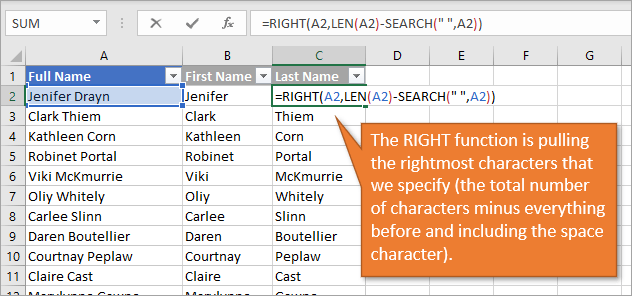
Note that we did not subtract 1 like we did before, because we want the space character included in the number that is being deducted from the total length.

Pros and Cons for Using Formulas to Split Cells

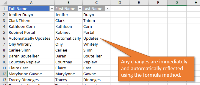
The one outstanding advantage to this method for splitting text is the automatic updates. When edits, additions, or deletions are made to the Full Name column, the First and Last names change as well. This is a big benefit compared to using Text to Columns, which requires you to completely repeat the process when changes are made. And even the Power Query method, though much simpler to update than Text to Columns, still requires a refresh to be manually selected.

Of course, one obvious disadvantage to this technique is that even though each of the four functions are relatively simple to understand, it takes some thought and time to combine them all and create formulas that work correctly. In other words, is not the easiest solution to implement of the three methods presented thus far.

Another disadvantage to consider is the fact that this only works for scenarios that have two names in the Full Name column. If you have data that includes middle names or two first names, the formula method isn't helpful without making some considerable modifications to the formulas. (Homework challenge! If you'd like to give that a try, please do so and let us know your results in the comments.) As we saw in the Power Query tutorial, you do in fact have the capability to pull out more than two names with that technique.

Ways to Split Text

Here are the links to the other posts on ways to split text:

• Split Cells with Text to Columns in Excel
• How to Split Text in Cells with Flash Fill in Excel
• How to Split Cells and Text in Excel with Power Query
• Split by Delimiter into Rows (and Columns) with Power Query

Conclusion

I hope you've learned something new from this post and that is helpful as you split data into separate columns. If you have questions or remarks, please leave a comment below!