Excel Challenge: Building a Dynamic Ordering System

Bottom line: Take on this Excel challenge to plan the perfect order for a team lunch or party.

Skill level: Beginner to Advanced

Download the Excel Files

Video Tutorial

Watch on YouTube & Subscribe to our Channel

Challenge Overview

In this Excel challenge, your task is to order pizzas for a party. You want to order just the right number of pizzas to stay on budget, satisfy all guests, and have the perfect amount of leftovers.

This challenge comes from the Weekly Challenges inside our Elevate Excel Training Program. The program also includes an all-access pass to our online course library, new AI Literacy for Excel course, community forum, live Q&A's and more.

Right now, you can try Elevate Excel for free during our limited time offer.

The Problem and Assumptions

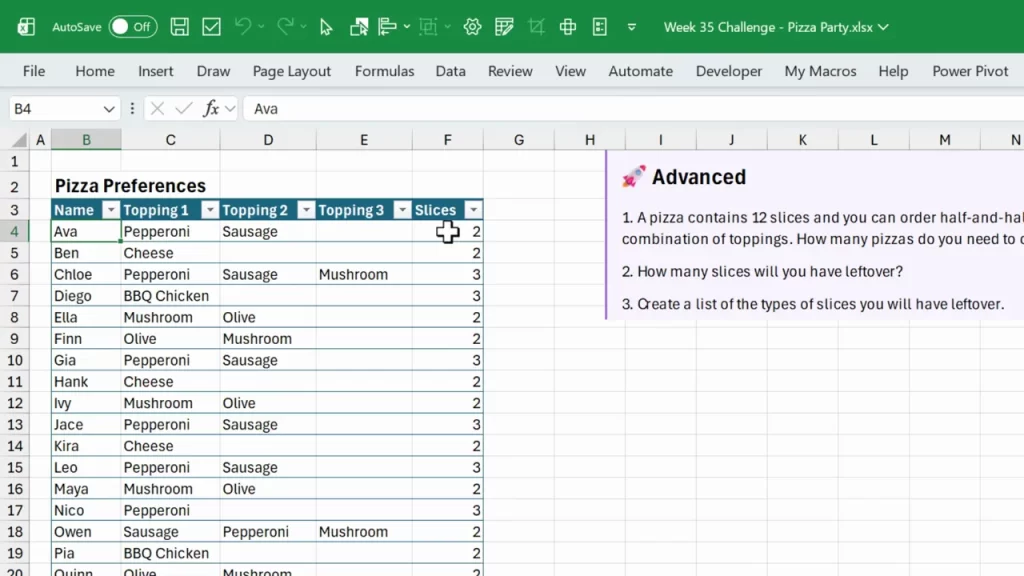
Start with a simple table of guests. Each row should include:

• Guest name
• Up to three preferred toppings
• Number of slices they will eat

Assumptions for this Excel Planning exercise:

• A pizza has 12 slices.
• Half-and-half pizzas are allowed. Each half contains 6 slices.
• Topping order should not change the pizza type. For example, mushroom + olive is the same as olive + mushroom.

Keep the inputs clean. Use dropdowns for toppings when possible. This reduces typos and makes grouping easier during analysis.

The Solution

The solution to the challenge is explained below.

It uses modern functions like TEXTJOIN, SORT, UNIQUE, SUMIF, ROUNDUP, and FILTER. Each section includes a screenshot to match the steps. Follow the numbered steps, and you will have an automated pizza planner that scales with party size.

1. Build a consistent pizza type column

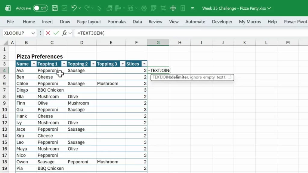
Create a column that represents each person’s pizza type. This column normalizes toppings and makes it possible to group identical pizzas.

Steps:

1. Use the TEXTJOIN function to combine the up to three topping cells into a single string.
2. Ignore empty topping cells so single- and double-topping pizzas work.
3. Sort the items in that row so topping order does not matter.

Example formula pattern:

=TEXTJOIN(", ", TRUE, [Topping1], [Topping2], [Topping3])

To normalize order, wrap the SORT function inside TEXTJOIN. Because toppings are laid out across a row, use the by_column argument:

=TEXTJOIN(", ", TRUE, SORT([ToppingRange],,TRUE))

This produces one value per row like Cheese or Olive, Mushroom. Use that column as the canonical pizza type for grouping.

2. Summarize slices per pizza type

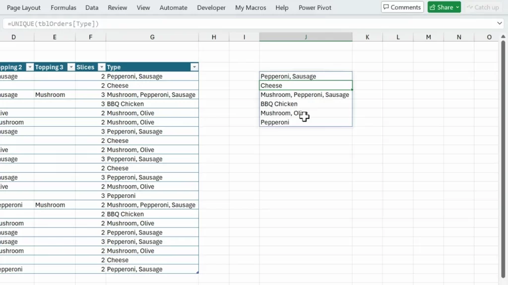
Now use a summary area to show all pizza types and total slices needed for each type. This is a key part of Excel planning: convert individual demands into aggregated demand.

Steps:

1. Use the UNIQUE function to list the distinct pizza types from the joined type column.
2. Use SUMIF to total the slices for each pizza type.

Example:

=UNIQUE([TypeColumn])

=SUMIF([TypeColumn], [UniqueType]#, [SlicesColumn])

Notes:

• Use the spill operator (#) when referencing a dynamic UNIQUE range in subsequent formulas.
• This approach works in most modern Excel versions. If you prefer, a pivot table or GROUP BY can be used instead. But UNIQUE + SUMIF keeps everything formula-driven and dynamic.

3. Convert slices to half-pizzas and full pizzas

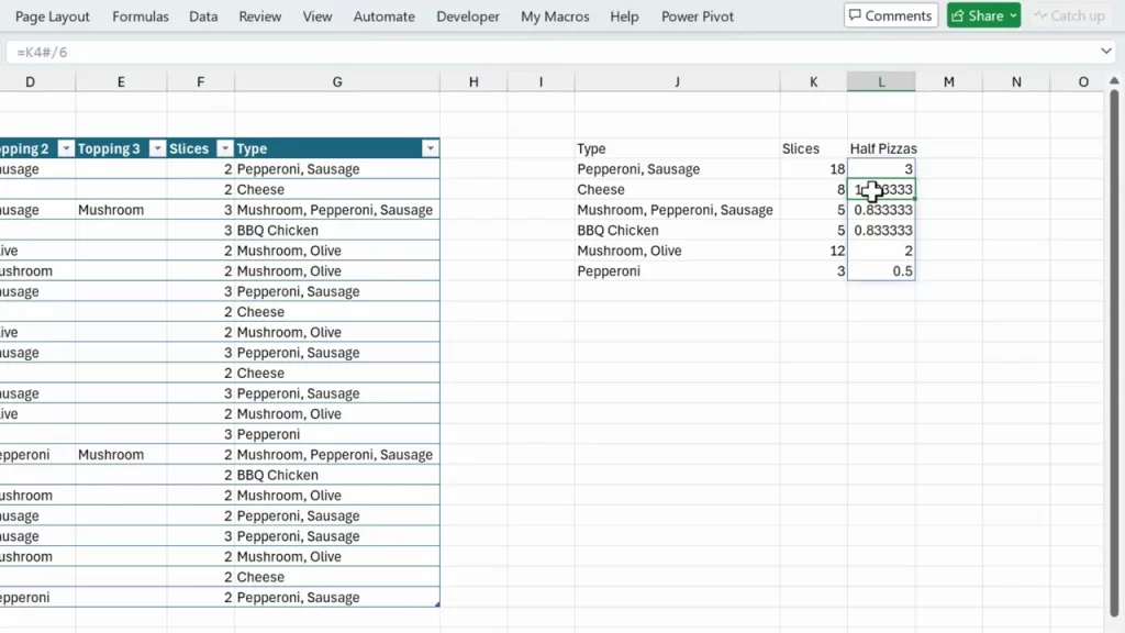
Because half-and-half pizzas are allowed, convert the total slices per pizza type into halves. Half a pizza equals 6 slices.

Steps:

1. Divide the slices per type by 6 to get the number of halves needed.
2. Round up that result because any fractional half still requires ordering a full half.
3. Sum the halves across all pizza types. Divide by 2 to convert halves to whole pizzas.

Formulas to use:

=ROUNDUP([SlicesPerType#]/6, 0)

=SUM([HalfPizzasRange#]) / 2

Why round up?

• If you need 1.2 halves, you must order 2 halves. ROUNDUP forces full-half counts.
• This ensures there are enough slices for each topping combination.

Excel Planning here helps avoid ordering too little. It gives a clear number of half pizzas for each topping and a total pizza count. If decimals remain after dividing halves by 2, that indicates an extra half pizza rather than a partial full pizza.

4. Calculate leftovers

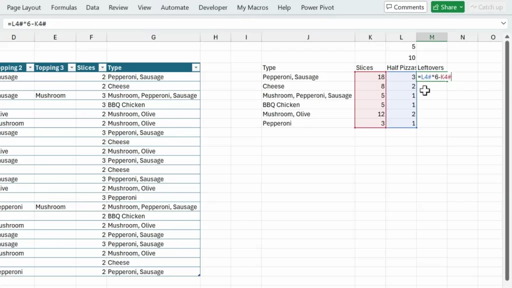
Leftovers are easy once you have the half counts. Each half contains 6 slices. Multiply halves by 6 and subtract the slices that guests will eat.

Formula:

LeftoversPerType = HalfPizzasPerType# * 6 - SlicesPerType#

Then sum across types to get total leftover slices.

Example outcome from a small party: nine leftover slices. That is useful for covering unexpected hunger or for next-day lunch.

Quick rules for Excel Planning and leftovers:

• Decide how many leftovers you want. If you prefer zero leftovers, adjust the rounding policy and be cautious.
• Leftover slices can help if a guest eats more than expected.

5. Advanced: Create a dynamic split-pizza order list

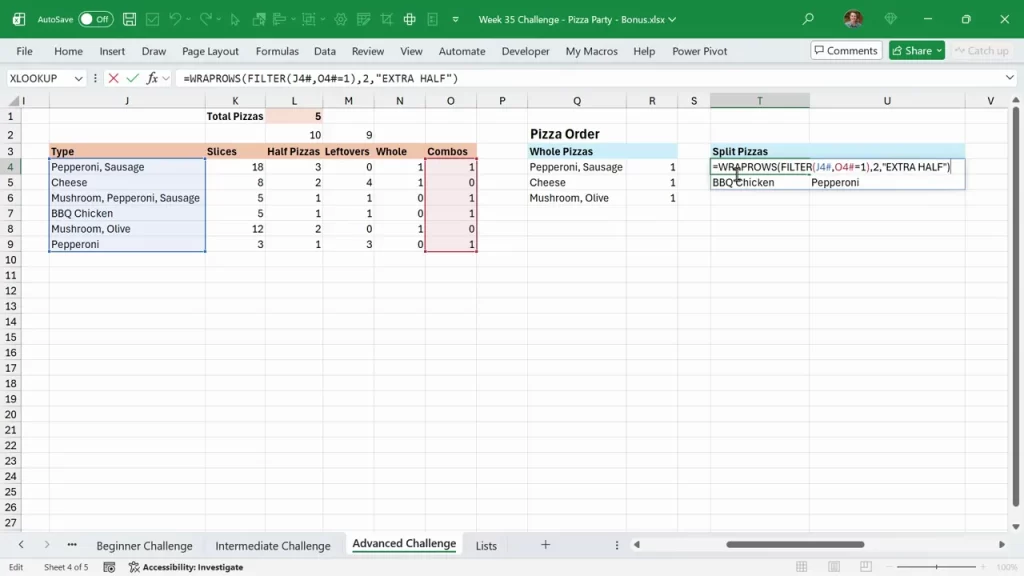
To make orders easier to place with a vendor, generate a list of which half goes with which topping. Use the FILTER function and dynamic arrays to build those lists automatically.

Concept:

• Start with the joined pizza types and their half counts.
• For any type with 2 halves, that represents one whole pizza. For an odd half count, one half will pair with another odd half to make a split pizza.
• Use FILTER to extract only halves that need pairing and list them side by side.

Benefits:

• Quick packing list for the pizza place.
• Visual confirmation of how halves will be combined.
• Automatic updates when any guest’s slice count changes.

Because dynamic arrays propagate automatically, changing a single cell in the guest table updates the entire order. That is powerful Excel Planning. For example, if a guest jumps to 22 slices, the sheet recalculates and shows the new 6.5 total pizzas and which half needs pairing.

Final Thoughts

Good Excel planning turns messy inputs into clear decisions. The pizza planner described here is a compact example of that approach. It replaces guesswork with formulas to give a precise count of halves, whole pizzas, and leftovers.

And ultimately, your guests will be satisfied. 😊

Try Elevate Excel Today

As I mentioned before, this challenge comes from the Weekly Challenges inside our Elevate Excel Training Program.

The program also includes

• An all-access pass to our online course library (over 22 courses)
• Community forum
• Live Q&A meetings
• Weekly Challenges
• New AI Literacy for Excel Course
• And a lot more

Right now you can try Elevate Excel for free during our limited time offer.