Bottom line: Learn the correct way to filter out zeros and numbers with the filter drop-down menus in Excel, and avoid embarrassing mistakes.
Skill level: Intermediate
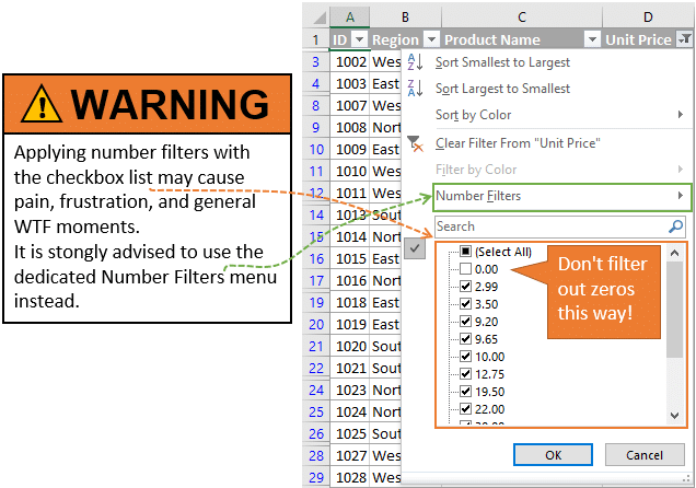
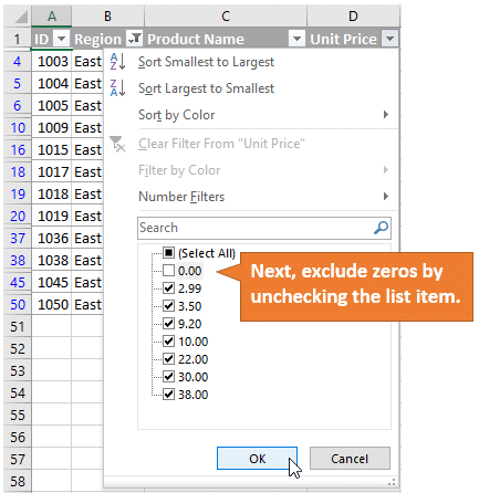
The image above shows a way to filter out numbers or zeros using the check boxes in the filter drop-down list. This way of applying number filters has gotten me in trouble. I have seen others make this common mistake too, and don't want it to happen to you. 🙂
Download Example File
Download the example file to follow along.
The Easy, But INCORRECT Way to Filter Out Zeros
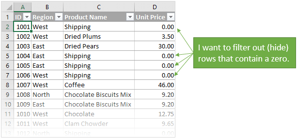
Often times we are working with a list or data set that contains a lot of zeros in a column. We might want to filter these zeros out to shorten the list, so that we only see numbers that are greater than or less than zero.
One easy way to do this is to uncheck the zero (0) item in the filter drop-down box.
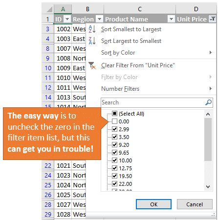
This does work, and will filter out (hide) the rows that contain zeros in the cells for the column. There won't be any issues if you only have that one column filtered.
However, problems arise when you have filters applied to more than one column.
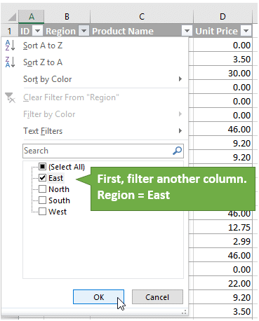
For example, let's say that we:
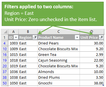
- First apply a filter to column B for the East Region.

- Then apply a filter to column D to exclude zeros by unchecking the zero item check box.

Everything is fine at this point.
We are seeing rows for the East Region where the Unit Price is not zero. This is our filter context.
Now, I want to clear the Region filter to view all Regions.
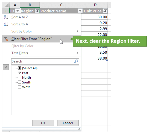
I assume that I should see rows for all Regions where the Unit Price is not zero.
WRONG!!!
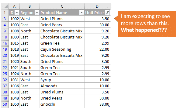
If we look at the filter drop-down for the Unit Price we can see that there are some amounts that are unchecked. That means that these rows are hidden, even though the amount is not zero.
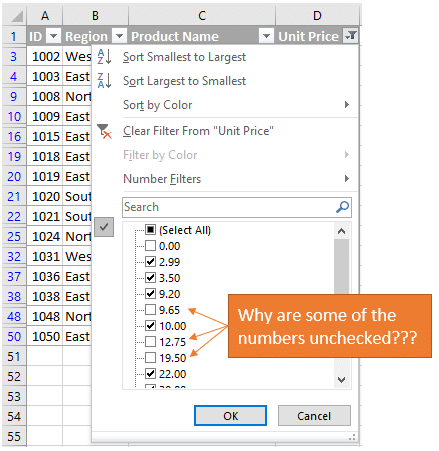
What's going on???
The Filter Drop-down List Checkboxes Explained
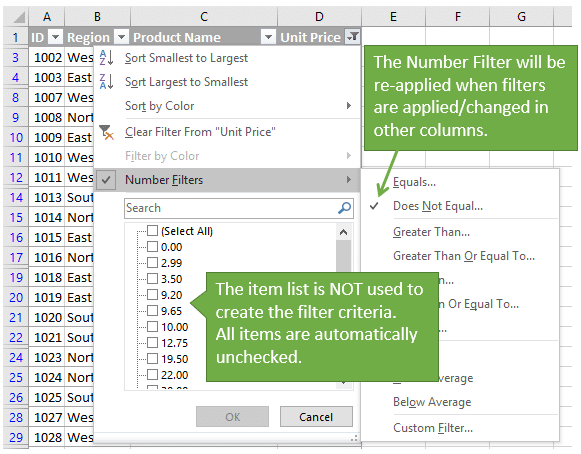
The filter list in the filter drop-down menu displays a list of unique items for that column (field). We can check or uncheck items in the list to apply filters and hide rows in the range/table.
When we uncheck one or more items, the filter creates a filter criteria to apply to the list. This filter criteria is a list of all the checked items. This is important.
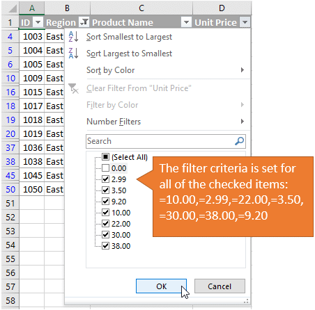
The filter criteria does NOT consider the unchecked items. Even if you have one item unchecked, and 1,000 items checked, the filter criteria will be for the 1,000 checked items.
In the example above, when I unchecked the zero in column D, the filter criteria became.
=10.00,=2.99,=22.00,=3.50,=30.00,=38.00,=9.20
I used a little VBA code to get the filter criteria.
Even though I meant to apply a filter to exclude zero, I actually applied a filter to include all the other numbers besides zero.
Since I had already applied a filter for the East Region, the Unit Price item list only contained numbers for the visible rows.
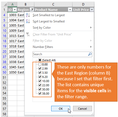
When we clear the filter in column B to show all Regions, the filter criteria for column D does NOT change. This means that there is still a filter applied for the numbers that are not zero for the East Region only.
Some of these numbers might also exist in rows for other regions, but overall it just becomes a meaningless mess. 🙂 This can lead to a lot of confusion when you are trying to tie out numbers or validate a summary report calculation.
So let's take a look at a safer approach.
The Correct Way to Filter Numbers
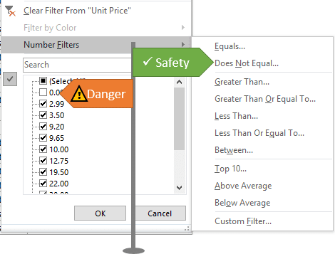
We saw how using the filter list checkboxes can get us in trouble when filtering numbers.
The safest way to filter numbers is by using the Number Filters menu on the filter list drop-down.
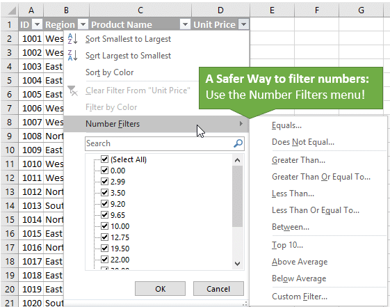
Selecting the Number Filters option will display a sub-menu with different number filter options (Equals, Does Not Equal, Greater Than, Less Than, Top 10, etc.)
Most of these commands open the Custom AutoFilter menu. This menu allows you to specify two criteria with an AND or OR condition.
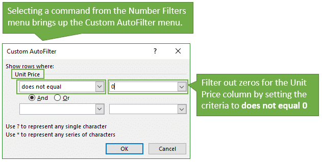
It is easy to create a filter to exclude zeros. We will set the filter criteria to “does not equal”, put a zero in the combobox to the right of the criteria, and press OK.
This sets a number filter with a criteria of “does not equal 0”:
<>0
The less than and greater than symbols together “<>” is the comparison operator for Not Equal, or the opposite of “=”.
This filter criteria helps us avoid the problem we experienced with the filter checkbox list.
Now when we clear or change the Region filter in column B, the number filter in column D will be re-applied to exclude all cells that contain a zero.
This is what we want. We don't have to go back to column D and re-select the checkboxes. The number filter will automatically be applied.
Keyboard Shortcuts for the Number Filters
The number filters take a few extra steps to apply, but it is well worth the time and effort if you are filtering multiple columns.
We can also use keyboard shortcuts to quickly apply a filter to exclude zeros.
With the header cell selected (the cell that contains the drop-down icon), press:
Alt+Down Arrow, F, N, 0, Enter
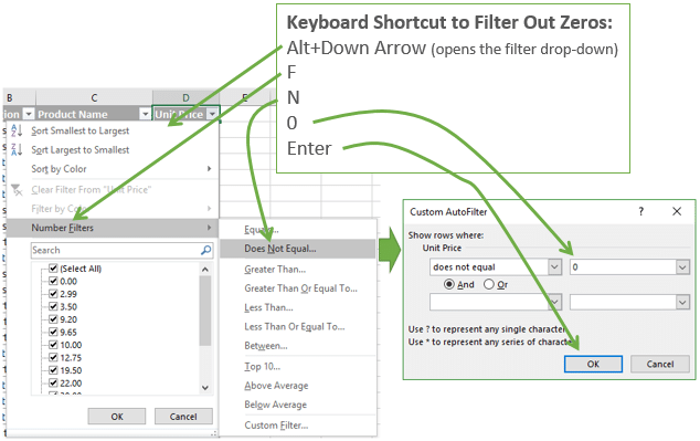
That is the keyboard shortcut to apply the number filter does not equal 0. There are many variations to this keyboard shortcut combination. Each of the underlined letters in the filter drop-down menu is the shortcut key for that menu item.
Checkout my article on 7 keyboard shortcuts for the filter drop-down menus that will save you a lot of time when working with filters. I also explain my favorite shortcut key to put the cursor in the Search box.
Conclusion
As we've seen, the filter drop-down item list can get us in trouble. I hope this article helps you avoid some of the mistakes I have made, along with the embarrassment… 🙂
In another article I will follow up with the VBA code and macro to get the filter criteria for the filter range or Table.
Please leave a comment below with any questions. Thanks!


What other tips do you have for filtering numbers? Please leave a comment below with any questions or suggestions. Thanks!
I was doing it the wrong way but not now. Thanks Will past this on to my friends.
Thanks Milt! It’s a hard habit to break, and I must admit that still use the checkboxes sometimes. Thanks for sharing! Have a good one! 🙂
Thanks Jon for the excellent explanation! This is very important to know! I’ll definitely share this!
Cheers,
Kevin
Thanks Kevin! I really appreciate that! 🙂
Thanks jon
Thanks Jon for your excellent tutorial! I have faced this problem yesterday. I have AR Aging excel sheet to filter customers horizontally excluding zero for invoices past due more than 30,60,90 days up to 180 days. How to solve this problem.
Best Regards,
Khaled Naser
Hi Khaled,
Great question! You might want to create a helper column that contains the max value of all the columns, then filter on that column.
It would probably be best if I could look at an example file, to make sure I fully understand your question. If you want to email me your file I would be happy to take a look. [email protected]
Thanks!
Hi Jon,
Great tip, will definitely pass this on.
Thanks Craig! I appreciate you sharing it. 🙂
Hi Jon
Thank you for your tutorial
I was not able to reproduce this using Excel 2013 french version
I am wondering if this is because I am not using same separator for numbers than your English version
Thank you
Hi Adel,
I’m sorry, which part were you trying to produce? I don’t believe you need comma separated values to apply the filter criteria.
Thanks!
Jon
This will help me great as need to filter zeros in AR calculation.Thanks and i will share with my team
Awesome! Thanks so much for sharing! 🙂
Good point but I suspect it’s only half the story.
Wouldn’t be true for all filters e.g. text, not just numbers.
Think conditional “To do list”.
Hi Mike,
Yes, the same theory can apply to text. It really applies to any time you are trying to “filter out” or exclude a value from the filter criteria, and the order in which you are filtering or clearing filters.
The example I gave was very simple, to make it easy to illustrate the point. However, we probably all have filter criteria that are much more complex. Hopefully this will get everyone thinking, and I will follow up with other articles on different scenarios.
Thanks for the comment, and have a good one!
Brilliant, thankyou. I have had exactly this problem this week.
Thanks Michelle! 🙂
Nice! I was actually unaware of this; however, so rarely do I go from two filters down to one filter or three filters down to two filters, etc. Normally I just toggle the filters off and then on again going from a table filtered by multiple columns to an unfiltered table. Definitely something to keep in mind though!
Thanks Ryan! I agree that clearing all filters is probably the safest way to go when multiple columns are filtered. Have a good one!
The first step was filter column D ( we are already without Zero) then we filter column B, at this point is not necessary “eliminate” zeros, because the list is already with amount > 0
When we clear the filter by Region, nothing happend. Anyway is interesting to learn another way. thank you!
ROSA
Hi Rosa,
The first step was applying a filter to a column with text (column B). If you apply that before filtering out zeros then you can get in trouble if you clear the filter on column B. This is a simple example, and can even more complex when more than two columns are filtered. I hope that helps. Thanks!
This is a wonderful post. I had never put together that the filter is additive. I mean I had, but it never really sank in until I read this. Nonetheless I did manage a rather in-depth post describing the many VBA Autofilter parameter settings which you and your readers might enjoy: http://yoursumbuddy.com/autofilter-vba-operator-parameters/
Thanks Doug! I know, I had to make the mistake a few times before I realized what was going on with the additive filters. Thanks for sharing the autofilter code. That is a great little solution for a common task! Have a good one!
Thanks for the great article! I consider myself an advanced Excel user, and I never knew this. I also appreciate the keyboard shortcut so I can easily write macros with filters.
Awesome! Thanks for letting me know Timothy!
This finally explains what has been driving me crazy when I use filters. I couldn’t figure out what I was doing wrong. I assume this logic applies with pivot table filters as well?
Thanks Wanda! Happy to hear it helped. Yes, the logic applies to filtering values in pivot tables as well. A lot will depend on the filters you have applied to each area in the pivot. The filtering options are different for the Filters area vs the Rows, Columns, and Values area. But this technique should help when filtering the Values area. Thanks again!
Hello Jon, why that filtering in Excel 0 and 0.00 are seen as different values. I tried filtering by zero 0, but number were formatted as 0.00 in a numeric field.
Thank you.
May-2017
filter: > -0,999999999 and < 0,000000001
Hi, I’ve searched your blog for my issue, but can’t find it. I’m using a version 2016 in Office 365. It’s a new computer. I’m trying to filter out numbers and it’s not finding the number. For example, if I type 2680 in the search, it returns nothing even though 2,680.00 is in the column. If I type 2,680 (with a comma) it will show up. I’ve never had to do that before. Is there a setting I can change so I can go back to typing 2680 and disregard commas. The same issue happens when I use the Number filtering. Thank you.