Bottom line: Learn how to convert dates stored as text to date values in Excel using Flash Fill. There are many possible solutions to this problem, so please leave a comment below explaining the technique that you would use.
Skill level: Intermediate
Live Training on Your Suggestions
Download the Excel file
Download the Excel file to follow along and complete the challenge.
Data Cleansing Challenge
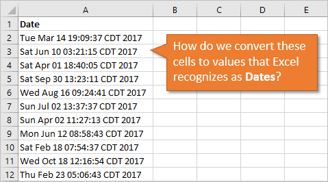
Mark, a member of The Pivot Ready Course, had a great question about converting text to dates. He has a data set exported from a system that contains a column with a date & time. Excel does not recognize these cells as a date data type. Therefore, he cannot sort the column or use it with the date grouping feature of a pivot table.
Here is the text for the date that you can copy/paste to Excel. You can also download the example file above.
Tue Mar 14 19:09:37 CDT 2017
So, how do we convert the text into a date that Excel recognizes?
There are several ways to go about this task in Excel. In the video above I share one solution using Flash Fill. I also explain how to determine if Excel recognizes the value as a date, so let's look at that first.
How To Tell If The Cell Contains A Date
We first need to determine if Excel is recognizing the value in the cell as text or a date.
Method #1: Number Format Drop-down Menu
Here's an easy way to figure it out the data type of the cell using the Number Format Menu:
- Select the cell.
- Click the Number Format drop-down on the Home tab of the ribbon.
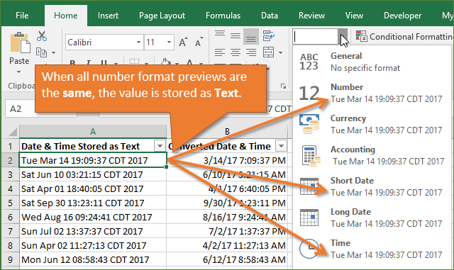
- If the preview of each number format has the same value as the cell contents, then it is Text.
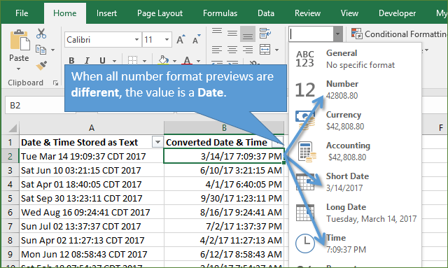
- If the preview changes for number format, then the cell is recognized as a Date.
The image below shows what we will see if the value is stored as Text.
And here is an image of the cell value that is recognized as a date.
Checkout my article and video on Dates in Excel to learn more. This is a very important concept that will help you cleanse your data and work with dates.
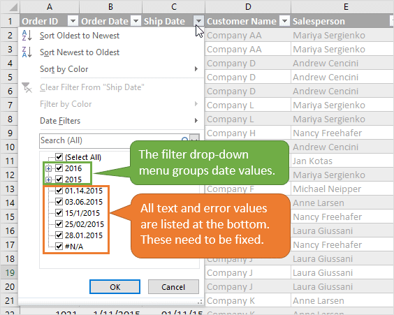
Method #2: Filter Drop-down Menu
Another way to see the data type is by using the filter drop-down menu.
In the image below you can see the filter list on the left is all text values. The column for the filter list on the right contains dates, and the date values in the filter list are grouped into Year, Month, Day, Minute, Hour, Second.
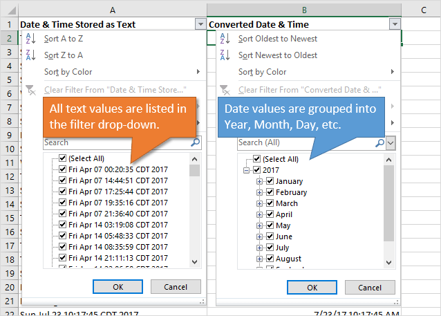
If you have some text at the bottom of the grouped dates, then those values will need to be converted to dates to use all the grouping features of a pivot table.
Convert Text to Dates with Flash Fill
Our challenge is to convert the text to a date value. There are several ways to solve this problem, and I'm looking forward to seeing your solution in the comments below.
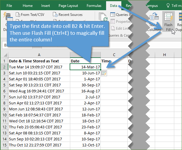
One simple way is to use the new Flash Fill feature. Flash Fill was introduced in Excel 2013 for Windows, and it's a really handy tool for data cleansing tasks.
Here's how to use Flash Fill to extract the date and time out of each cell:
- Select a blank cell to the right of the cell that contains the date stored as text. If the adjacent cell isn't blank, insert a blank column or copy the column to a blank sheet.
- Type the date that is in the cell and press Enter. In the example in the video I typed the following into the cell: Mar 14, 2017
- Click the Flash Fill button on the data tab of the Ribbon. The keyboard shortcut for Flash Fill is Ctrl+E.
- Flash Fill will find the date in each cell in column A and fill it down column B.
Checkout the video above to see it in action.
We can use the same technique to extract the Time into column C.
- Double-click cell A2 to edit it, select the text for the time, and copy it.
- Paste the time in cell C2. Excel automatically recognizes this as a time value.
- Press Ctrl+E or the Flash Fill button to fill the entire column with the times from column A.
Finally, we might want to combined the date and time into one column. We can do with a formula in column E that sums the date and time value from B2 & C2.
Excel should automatically change the number format to a date & time format. If you see a number like 42808.80, then you can change the number format to view it as a date and time. See the video above for details.
Checkout my article and video on how dates work in Excel to learn more about how dates are numbers formatted as dates. I also have an article on how to get the day name for a date
How Would You Convert This Text to a Date?
There are many ways to go about this challenge in Excel, and I want to know how you would solve it. Please leave a comment below with the technique you would use.
There are NO wrong answers here, and this will be a great opportunity to learn from everyone, so don't be afraid to share your answer. 🙂
I will create a follow-up video with some of the most common responses. Thank you!


The Flash Fill is clearly the most elegant (and fastest). Another method:
1. Use Text to Columns to get separate columns for each “word:” Tue Mar 14 19:09:37 CDT 2017
2. Use concatenation to create a “pseudo-date” (one that looks like a date but is text): =B2&” “&C2&”, “&F2 = Mar 14, 2017
3. Multiply the result by 1 to convert it into a date. (Excel usually takes numbers formatted as text that are used in a formula and converts them into numbers.)
4. Time converts directly. Add the date and time columns and format as you describe.
This was an opportunity for me to test my Power Query knowledge so I went for it.
1. Load the table into the Power Query Editor.
2. Promote the first row as header
3. Split the column into columns by “space” delimiter
4. Delete the columns not needed (day names and CDT columns)
5. Move year column (2017) left to shift time column to the right
6. Select remaining columns and merge to get desired result.
7. Close and load.
Love this solution! Fastest one for me. I have Excel 2010 so don’t have the flash fill feature, but using Power Query seemed so much faster than the Flash Fill option. I was finished in just about 1 minute following your steps.
Jon,
Excellent source of information I will use this method for my job, to save time.
Does excel calculate the day of week when entered the date???
Sid,
Yes. You can view the date as the day of week by choosing custom format dddd.
Mt
I did not want to use a separate table for lookups. Originally parsed out step by step in columns, but then reduced to this in a single cell:
with the original text in cell A4
DATEVALUE(TEXTJOIN(” “, TRUE,(LEFT(RIGHT(A4,LEN(A4)-4),SEARCH(” “,RIGHT(A4,LEN(A4)-4),5))), “,”,RIGHT(RIGHT(A4,LEN(A4)-4),4)))+TIMEVALUE(MID(RIGHT(A4,LEN(A4)-4),SEARCH(” “,RIGHT(A4,LEN(A4)-4),6)+1,8))
This gives an excel date-time value, which formatted with “m/d/yy h:mm:ss AM/PM” gives the display desired.
Until this, I never appreciated how useful it is that the time part of a date-time is a decimal value, so could just be added to the date part.
I used =DATEVALUE(TEXT(MID(A2,9,2)&” “&MID(A2,5,3)&” “&RIGHT(A2,4),”mm/dd/yyyy”))+TIMEVALUE(MID(A2,12,8))
=MID(REPLACE(A1,11,,CONCATENATE(“, “,RIGHT(A1,4))),5,21)
Goes from: Tue Mar 14 19:09:37 CDT 2017
To: Mar 14, 2017 19:09:37
Then: =DATEVALUE(LEFT(B1,12))+TIMEVALUE(MID(B1,14,8)) with the correct date format for the cell, 3/14/17 7:09:37 PM
=DATEVALUE(MID(A1,9,2)&”-“&MID(A1,5,3)&”-“&RIGHT(A1,4))
Great brain teaser, thanks! 😉
My answer is maybe not the fastest one, but it works:
1. column – MONTH =VLOOKUP(MID(A2,5,3),Months!A:B,2,0). I’ve created one additional sheet “Months” with the names of months in one column and numbers in another
2. column – YEAR /=RIGHT(A2,4)*1/
3. column – DAY /=MID(A2,9,2)*1/
4. column – DATE /=DATE(C2,B2,D2)/
5. column – TIME /=MID(A2,12,8)*1/
6. column – Converted Date & Time /=E2+F2/
7. column – Check /=VLOOKUP(A2,Explanation!A:B,2,0)-G2/ and all the results were zeros, yeeees! 😉
Great brain teaser, thanks! 😀
My answer is maybe not the fastest one but it works:
Column B: MONTH /=VLOOKUP(MID(A2,5,3),Months!A:B,2,0)/ I’ve added additional sheet “Months” with names in one column and numbers in another
Column C: YEAR /=RIGHT(A2,4)*1/
Column D: DAY /=MID(A2,9,2)*1/
Column E: DATE /=DATE(C2,B2,D2)/
Column F: TIME /=MID(A2,12,8)*1/
Column G: Converted Date & Time /=E2+F2/
Column H: Check /=VLOOKUP(A2,Explanation!A:B,2,0)-G2/ I’ve checked all the results with “Explanation” sheet and got all zeros, yeeeessss! 😀
Wow that was way cool and so fast/easy! Thanks for sharing Flash Fill!
I had an extra problem using the Dutch version of Excel: the name of the month is not recognized!
I first used text to columns (fixed width) to separate, skipping the name of the day and CDT.
Then I moved the column with the time to be the last column.
Result:
A B C D
2 Mar 14 2017 19:09:37
3 Jun 10 2017 03:21:15
etc.
Then I made a table for numbering the names of the months in 2 columns
M N
1 Jan 1
2 Feb 2
3 …
Then I used the DATE-function to create a date from the Year-column, the Month-nale (using Vlookup to change the name into a value) and the Day-column.
=DATE(C2;VLOOKUP(A2;@M$1:$N$12;2;FALSE);B2)
I copied that column down for the whole table.
Select the column with the created dates, copy it, paste values in the same place.
Then delete the columns A,B and C and the lookup table.
How about this…
=REPLACE(MID(SUBSTITUTE(A2,”CDT “, “”),5,99),7,0,”, “&RIGHT(A2,4))
EDIT… I forgot the +0
=REPLACE(MID(SUBSTITUTE(A2,”CDT “, “”),5,99), 7,0,”, “&RIGHT(A2,4))+0
And not to mention, apply custom format to the result
Bravo, I was trying to figure out a SUBSTITUTE type formula. Works perfectly. I have much to learn!
Hi,
Here is one solution, which does not depend on regional settings:
=DATE(RIGHT(A3,4),MATCH(MID(A3,5,3),{“Jan”,”Feb”,”Mar”,”Apr”,”May”,”Jun”,”Jul”,”Aug”,”Sep”,”Oct”,”Nov”,”Dec”},0),MID(A3,9,2))+VALUE(MID(A3,12,8))
Match gives you an index number based on the three letter found in text from the 3rd to the 5th position defined by MID.
Cheers
Attila
(Excel 2003)
First, I extracted day, month, year, time:
“DAY” (B2) =VALUE(MID(A2,9,2))
“MONTH” (C2) =MID(A2,5,3)
“YEAR” (D2) =VALUE(RIGHT(A2,4))
“TIME” (E2) =MID(A2,12,8)
Next, calculated the date and time values:
“DATEVALUE” (F2) =DATEVALUE(CONCATENATE(B2,”-“,C2,”-“,D2))
“TIMEVALUE” (G2) =TIMEVALUE(E2)
Finally, combined the two:
“DATE & TIME” (H2) =F2+G2
Apparently, there could have been less formulas but I prefer small steps at a time.
(Excel 2003)
First, I extracted texts for day, month, year, and time:
“DAY” (B2) =MID(A2,9,2)
“MONTH” (C2) =MID(A2,5,3)
“YEAR” (D2) =RIGHT(A2,4)
“TIME” (E2) =MID(A2,12,8)
Next, calculated the date and time values:
“DATEVALUE” (F2) =DATEVALUE(CONCATENATE(B2,”-“,C2,”-“,D2))
“TIMEVALUE” (G2) =TIMEVALUE(E2)
Finally, combined the two:
“DATE & TIME” (H2) =F2+G2
Apparently, there could have been less formulas but I prefer small steps at a time.
Months
Jan 1
Feb 2
Mar 3
Apr 4
May 5
Jun 6
Jul 7
Aug 8
Sep 9
Oct 10
Nov 11
Dec 12
=LEFT(A10;10)&” “&RIGHT(A10;4)
=(MID(A2;12;8))*1
=((MID(B2;9;2)&”/”&VLOOKUP(MID(B2;5;3);Months;2;0)&”/”&RIGHT(B2;4))*1)+C2
Flash fill is fine, but with these data it works. But if there are more years it will not work. Change some of the years into 2016 of 2018 and it will not work….
Workaround:
Start with typing the year, then the month and then the day (2017-Mar-14)in a new column.
Use Flash fill
End with:
Select the column and choose Data > Text to Columns. Then only change the last step selecting Date = YMD and it will work.
Hi John
I would personally do something like this:
=DATE(RIGHT(B3,4),MONTH(DATEVALUE(MID(B3,FIND(” “,B3)+1,3)&” 1″)),MID(B3,9,2))+TIMEVALUE(MID(B3,FIND(” “,B3,10)+1,8))
and format the cell as:
m/dd/yy h:mm:ss AM/PM
Peace.
Renier
I first used the formula =DATEVALUE(MID(A2,9,2)&MID(A2,5,3)&RIGHT(A2,4))+TIMEVALUE(MID(A2,12,8))
I then had a go with Powerquery which is nice and neat.
The method I used within PowerQuery was:
1 convert the raw data to a table (“Tbl_RawData”)
2 import using Data / From Table Range
3 Split the data by Delimiter “Space” all occurrences
4 Merge the new columns containing Day, Month, Year & time columns
5 Change the new columns data type to Date & Time
6 Finally, I renamed the Query to “Process raw dates”
7 “Close and Load to”
The contents of the Editor is below:
let
Source = Excel.CurrentWorkbook(){[Name=”Tbl_RawData”]}[Content],
#”Changed Type” = Table.TransformColumnTypes(Source,{{“Date & Time Stored as Text”, type text}}),
#”Split Column by Delimiter” = Table.SplitColumn(#”Changed Type”, “Date & Time Stored as Text”, Splitter.SplitTextByDelimiter(” “, QuoteStyle.Csv), {“Date & Time Stored as Text.1”, “Date & Time Stored as Text.2”, “Date & Time Stored as Text.3”, “Date & Time Stored as Text.4”, “Date & Time Stored as Text.5”, “Date & Time Stored as Text.6″}),
#”Changed Type1″ = Table.TransformColumnTypes(#”Split Column by Delimiter”,{{“Date & Time Stored as Text.1”, type text}, {“Date & Time Stored as Text.2”, type text}, {“Date & Time Stored as Text.3”, Int64.Type}, {“Date & Time Stored as Text.4”, type time}, {“Date & Time Stored as Text.5”, type text}, {“Date & Time Stored as Text.6″, Int64.Type}}),
#”Merged Columns” = Table.CombineColumns(Table.TransformColumnTypes(#”Changed Type1″, {{“Date & Time Stored as Text.3”, type text}, {“Date & Time Stored as Text.6”, type text}, {“Date & Time Stored as Text.4”, type text}}, “en-GB”),{“Date & Time Stored as Text.3”, “Date & Time Stored as Text.2”, “Date & Time Stored as Text.6”, “Date & Time Stored as Text.4″},Combiner.CombineTextByDelimiter(” “, QuoteStyle.None),”Merged”),
#”Changed Type2″ = Table.TransformColumnTypes(#”Merged Columns”,{{“Merged”, type datetime}}),
#”Removed Columns” = Table.RemoveColumns(#”Changed Type2″,{“Date & Time Stored as Text.1”, “Date & Time Stored as Text.5″}),
#”Renamed Columns” = Table.RenameColumns(#”Removed Columns”,{{“Merged”, “Date & Time”}})
in
#”Renamed Columns”
Dear Sir,
i need your help in vba macros from beginning.you would be help me
Reading through these responses inspired me to think about this problem more, and I came up with what I think is a very elegant solution to this problem. Since we know that these dates are a fixed length we could do something like this (assume that this formula is written in cell C2 for the first row of data and can then be auto-filled to the bottom):
=RIGHT(REPLACE(A2,11,13,”,”),12)+MID(A2,12,7)
Because you use the “+” operator, you don’t even have to convert the range with any “*1” or any of that business. AND, It would even be possible to make this solution work with FIND() or SEARCH() for text date-timestamps that are not fixed length!
Thanks everyone for the inspiration!!
I did Text to Columns since all the dates were fixed length.
Column 1, Row 2 = Tue
Column 2, Row 2 = 14-Mar
Column 3, Row 2 = 19:09:37
Column 4, Row 2 = CDT
Column 5, Row 2 = 2017
Column 7 = ‘=TEXT(B2,”mm/dd”)&”/”&E2 RESULT is 03/14/2017
The Time stands alone in column 3
Went with different idea uses current year only but it seems to work
Highlight column A
DATA
Text to Columns
Fixed Width
Next
Remove or move lines
leaving line on left side of month
leaving line on right side of time
This leaves three columns Click Next
1st column mark do not import
3rd column mark do not import
Click Finish
Highlight column A
Home Tab format cells
Custom
Select or Type
[$-409]m/d/yy h:mm:ss AM/PM;@
Rename A1 if needed
Done
Hi Jon,
I tried with a VBA approach:
Sub ConvertTime()
‘ Set data range
Dim rg As Range, c As Range
Set rg = Range(“A1”).CurrentRegion
‘ Move through range
For Each c In rg.Cells
‘ Add value to variable
Dim sTime As String
sTime = Range(“A” & c.Row).Value
‘ Split into array
Dim vArrTime As Variant
vArrTime = Split(sTime, ” “)
‘ Get date and time from array
Dim sMyTime As Date
sMyTime = vArrTime(5) & “-” & vArrTime(1) & “-” & vArrTime(2) & ” ” & vArrTime(3)
‘ Print date and time and format it
With Range(“B” & c.Row)
.Value = sMyTime
.NumberFormat = “yyyy/mm/dd hh:mm:ss”
End With
Next c
End Sub
Thanks for the “homework” assignment; it got me back to my Excel training. I wanted to solve it using my limited knowledge without looking anything up. So I did it in a totally convoluted backward way that I could not even begin to explain here (it involved 19 columns), but in the end I got an automated worksheet that allowed me to just copy the first row down. But it was a good exercise and forced me to think in a logical way. When I looked at the much easier ways that other were able to do it, it proved that although there is more than one way to skin a cat in Excel, it’s best to know the shortest way!
Jon,
First I used Power Query similar to Ali Kassie.
Then I used the following formula:
=DATEVALUE(MID(A2,5,6)&”, “&RIGHT(A2,4))+TIMEVALUE(MID(A2,12,8))
change formatting to Custom m/d/yyyy h:mm AM/PM.
Thanks for the challenge!
Mt
Hi Jon,
First I tried Power Query similar to Ali Kassie.
Then, since I like formulas, I placed the following:
=DATEVALUE(MID(A2,5,6)&”, “&RIGHT(A2,4))+TIMEVALUE(MID(A2,12,8))
change formatting to Custom m/d/yyyy h:mm AM/PM
Thanks for the challenge!
Mt
Thks Jon for this tips.
But if one of the year is other than 2017 (say 2016), it doesn’t take year (2016) when using flash fill.It reports year 2017 throughout!
Thks Jon for coming back on this issue.
I used:
=DATE(RIGHT(A2,4),MONTH(DATEVALUE(MID(A2,5,3)&”1″)),MID(A2,9,2)) + TIME(MID(A2,12,2),MID(A2,15,2),MID(A2,18,2))
A bit long but very intuitive, I think.
Henk,
I found at least one shortcut in your formula. Once you have a date, you can add in the text for the time and it will translate it automatically.
=DATE(RIGHT(A2,4),MONTH(DATEVALUE(MID(A2,5,3)&”1″)),MID(A2,9,2)) + MID(A2,12,8)
=VALUE(MID(REPLACE(A2,11,13,”,”),5,12)) then change formatting to desired date format
I like this solution. It was not my intuitive process, so I can add this to possible solutions in the future. I also took it one step further and added the time into the formula.
=VALUE(MID(REPLACE(A2,11,13,”,”),5,12))+(MID(A2,12,8))
I also went woth VBA:
Function text2datetime(text$)
jaar$ = Right$(text$, 4)
maand$ = LCase$(Mid$(text$, 5, 3))
Select Case maand$
Case “jan”
maand$ = “01”
Case “feb”
maand$ = “02”
Case “mar”
maand$ = “03”
Case “apr”
maand$ = “04”
Case “may”
maand$ = “05”
Case “jun”
maand$ = “06”
Case “jul”
maand$ = “07”
Case “aug”
maand$ = “08”
Case “sep”
maand$ = “09”
Case “oct”
maand$ = “10”
Case “nov”
maand$ = “11”
Case “dec”
maand$ = “12”
Case Else
maand$ = “01”
End Select
Dag$ = Mid$(text$, 9, 2)
tijd$ = Mid$(text$, 12, 8)
datum$ = Dag$ & “/” & maand$ & “/” & jaar$
text2datetime = DateValue(datum$) + TimeValue(tijd$)
End Function
Jon,
I would tackle this using a function to pass the date-string variable to an array in a similar manner to the ConvertTime sub procedure suggested earlier.
Function fConvertTS(sDateString as String) as Date
Dim arrTS asVariant
arrTS = Split(sDateString,” “)
fConvertTS = DateValue(arrTS(1) & ” ” & arrTS(2) & ” ” & arrTS(5))
fConvertTS = fConvertTS + TimeValue(arrTS(3))
End Function
Looks like I am late to this conversation but…
I chose Text to Columns because of my limited knowledge of Excel.
I first selected the entire Column A of data excluding the header
Clicked on the Data Tab and then Text to Columns
In Step 1 of the Text to Columns, I selected Delimited and then Next
In Step 2 I chose “Space” as the delimiter and then Next
In Step 3 I chose “General”, then selected the 1st column and clicked on “Do not import column (skip)”, then selected the 5th column and clicked on “Do not import column (skip)”, and then Finish. Skipping those two columns just saves space.
Another option in Step 3 is “Destination”. I chose cell B2 just to preserve the original data while playing but it defaults to the original cell which in this case was A2 and although it does not list all of the cells highlighted below A2 they are included.
Now I have the month in Column B, day in Column C, time in Column D, and year in Column E.
I placed the following formula in Column F =SUM(DATE(E2,MONTH(1&B2),C2),D2).
You then use formatting to to see the date and time however suits you.
I chose a custom format “dddd mmm, dd yyyy hh:mm:ss” just for fun because it closely simulates the original text.
Obviously this would not work in those areas that do not recognize 3 letter month abbreviations but that is not part of this challenge.
After reading through these answers I really like the way Kent approached it. Very simple.
“Kent – November 16, 2017
Reading through these responses inspired me to think about this problem more, and I came up with what I think is a very elegant solution to this problem. Since we know that these dates are a fixed length we could do something like this (assume that this formula is written in cell C2 for the first row of data and can then be auto-filled to the bottom):
=RIGHT(REPLACE(A2,11,13,”,”),12)+MID(A2,12,7)
Because you use the “+” operator, you don’t even have to convert the range with any “*1” or any of that business. AND, It would even be possible to make this solution work with FIND() or SEARCH() for text date-timestamps that are not fixed length!
Thanks everyone for the inspiration!!”
how to get a copy of excel software thanks
Hi Jon,
Regarding Kent’s post on 11/16/17, I’m trying to figure out what the 12 is in his formula =RIGHT(REPLACE(A2,11,13,”,”),12)+MID(A2,12,7). I deleted it to see what would happen and it changes the year from 2017 to 1900. I tried 11 and got an error. I was unfamiliar with the REPLACE and MID formulas so I looked them up and played with them today. Nice to know!
Thank you.
Pam
I’ve built an amortization table and have dates as column headers.
1/1/2019, 2/1/2019, 3/1/2019,…
In another table I have Start Date and End Date columns. I’ve built a formula that essentially says, =IF(AND(1/1/2019 is > Start Date, 1/1/2019 < End Date),"TRUE", "")
So if it's between the start and end date I want a "TRUE" result.
This formula works fine when I have my data in just a range. (as you'll see in the file).
The second I turned that range into a table the formula gave me a false reading (because the dates in the column headers are now acting as TEXT and not DATES, despite me changing the format to date).
How can I fix this or workaround it?