5 Excel Functions That Replace 41 Others

Imagine you had to pick only 5 Excel Functions to solve most spreadsheet problems. Which ones would you keep?

I picked five functions that together replace a large number of smaller, niche functions. These choices focus on common tasks: lookups, logical tests, statistics, reporting, formatting, and data cleanup.

Video Tutorial

Watch on YouTube & Subscribe to our Channel

Download the Excel File

How I chose the 5 Excel Functions

My goal was simple. Pick functions that handle everyday data-analysis work. Each function should be versatile and combine multiple tasks into one formula.

I grouped needs into five categories. Each category gets a single function that handles most scenarios. That makes it easier to learn and to build reliable spreadsheets.

1. FILTER — The lookup plus logical swiss army knife

FILTER is the single function I use for lookups and many logical tests. It returns matching rows or values from an array based on criteria you set.

Why FILTER makes the cut

• Returns all matching results instead of just the first match.
• Handles multiple criteria using simple expressions and arithmetic for AND logic.
• Works as a dynamic range, so results auto-spill and update automatically.
• Can be easier to read and understand for some users, compared to XLOOKUP or VLOOKUP.
• The formula is short and only requires two arguments (return array, filter criteria).

=FILTER(I5:J20,G5:G20=B10)

Common uses

Here are typical scenarios where FILTER replaces other functions.

1. Lookup multiple rows for a customer and return several columns. Use FILTER instead of XLOOKUP when duplicates matter.
2. Implement tiered logic. For example, find which bonus tier a sales amount falls into by testing min and max columns.
3. Combine with other functions to create dynamic reports and extracts.

FILTER for Logical Tests

Filter can also be used in place of logical functions like IF or IFS. It can even handle AND and OR logic for multiple conditions.

The filter criteria below tests if the sales amount is greater than or equal to values in the minimum range and less than or equal to values in the maximum range, and returns the bonus amount.

(SalesAmount>=MinRange)*(SalesAmount<=MaxRange)

FILTER is a very versatile function that should be in every Excel user's tool belt.

2. AGGREGATE — One function to handle most statistical needs

AGGREGATE is the statistical workhorse I chose. It handles sum, average, count, and many other calculations, and it includes options to ignore hidden rows and errors.

Why AGGREGATE belongs in the 5 Excel Functions

• Supports many operations via a function number parameter.
• Can ignore hidden rows, errors, or nested subtotal/aggregate results.
• Works well inside tables and filtered views.

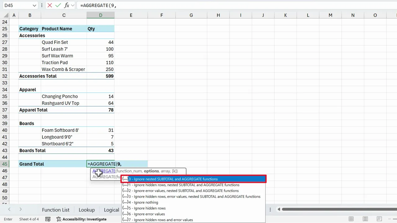
How AGGREGATE works

AGGREGATE takes a function number, an option number for what to ignore, and the array or range. The option lets you choose whether to ignore hidden rows, errors, or nested functions.

When to prefer AGGREGATE

• When you need calculations that respect filters and hidden rows.
• When your worksheet contains subtotal rows and you need to avoid double counting.
• When you want one formula to replace a set of SUM, AVERAGE, COUNT, SMALL, LARGE, etc.

Limitations

AGGREGATE can feel heavy when you only need a simple SUM or COUNT.

3. PIVOTBY — Build dynamic summary reports with a formula

PIVOTBY creates pivot-like summaries inside the grid. It builds cross-tab reports with a single function. It returns unique row and column headers and performs aggregation for each intersection.

Why PIVOTBY is part of the 5 Excel Functions

• Generates a pivot-style table with formulas instead of the PivotTable tool.
• Combines the work of UNIQUE, SUMIFS, and manual layout into one function call.
• Supports sorting and total rows with minimal setup.

Practical benefits

• Quickly prototype a report without creating a PivotTable object.
• Use in dashboards where formulas are preferable to PivotTables.
• Works well with dynamic data that changes shape often.

When to still use a PivotTable

PivotTables are powerful and user-friendly. They are still the best choice for complex, interactive reporting. Use PIVOTBY when you want formula-based outputs or programmatic control inside the worksheet.

4. TEXT — Formatting, grouping, and linked labels

TEXT converts numbers and dates into custom text formats. It is surprisingly flexible for grouping by month, producing labels, and creating formatted strings on dashboards.

Why TEXT makes the shortlist of 5 Excel Functions

• Extract month numbers, month names, weekdays, or years using number formats.
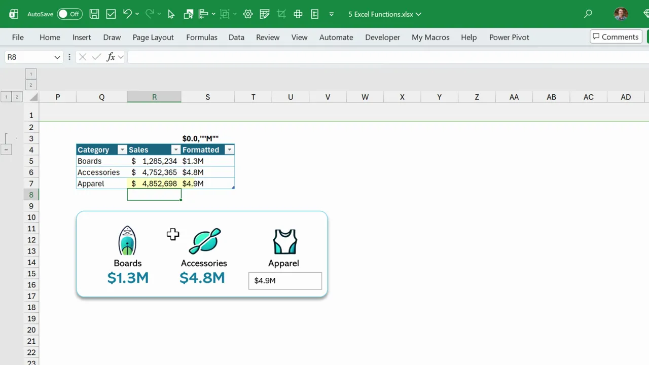
• Format numbers to show millions, thousands, currency, or other custom views.
• Produce readable labels for charts and text boxes that are linked to cell values.

Examples

1. Return month number: =TEXT(A2,”M”)
2. Return month name: =TEXT(A2,”mmmm”)
3. Format millions: =TEXT(Sales,”#,##0,,””M”””)

You can link a text box to a formatted cell so the visual label updates automatically. That is handy for scorecards and dashboards.

Tips

• Keep formatting codes in a reference row so you can reuse them quickly.
• Remember TEXT returns text, so use VALUE() or multiply by 1 if you need to convert back to a number.

5. REGEXEXTRACT — Clean and parse text with patterns

REGEXEXTRACT pulls parts of text using regular expressions. It replaces many text functions by matching patterns rather than relying on position.

Why REGEXEXTRACT is one of the 5 Excel Functions

• Extracts first or last names, company names, zip codes, and more.
• Can trim trailing spaces and find numbers inside long text strings.
• Combines the roles of TEXTBEFORE, TEXTAFTER, TEXTSPLIT, and TRIM in many cases.

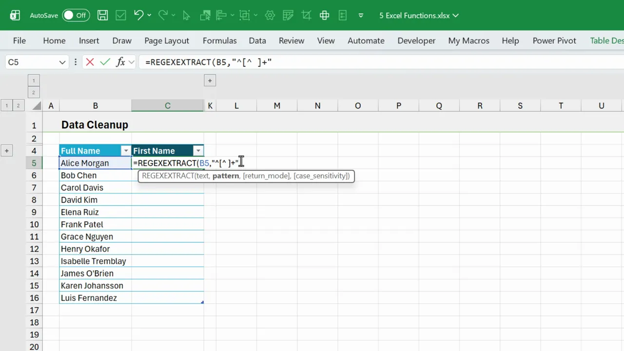
How to use REGEXEXTRACT

1. Type =REGEXEXTRACT(
2. Select the text cell you want to parse.
3. Provide the regular expression pattern in quotes or via a helper cell.
4. Close and press Enter. The matching group returns the extract.

For example, to get the first name before the first space you could use a pattern that captures characters up to the space. If building the pattern feels hard, there are quick ways to get started.

How to build patterns faster

• Use an AI assistant to generate regex patterns from a short description of the data.
• Create a library of common patterns and store them in a small table for reuse.
• Test patterns on sample strings to ensure they match the parts you expect.

REGEX brings a small learning curve, but it pays off with major flexibility for messy data. Plus, we can have AI write the regex codes and patterns for us.

Final thoughts on the 5 Excel Functions

Choosing only 5 Excel Functions forces you to pick versatile tools. FILTER, AGGREGATE, PIVOTBY, TEXT, and REGEXEXTRACT cover lookups, statistics, reporting, formatting, and cleanup.

They are not perfect for every edge case. But together they replace many niche functions and reduce complexity. Learning these five gives a powerful foundation for everyday spreadsheet work.

Download the Excel workbook from the section at the top to see the full list of functions that these 5 replace.

Which five would you choose? Share your list and a short reason.

Thanks so much!