Tips & Tricks for Writing CUBEVALUE Formulas

Imagine it's a hot summer day and you are enjoying a nice cold drink at your favorite spot.  What's one thing that will make that drink extra refreshing? Ice cubes! The CUBE functions in Excel are like the ice cubes of the PowerPivot beverage.  They are not required, but just add an element to the drink that makes it so much better.

Once you get to know the CUBE functions you will use them often.  And for good reason.  They allow you to query data from your PowerPivot model outside of a PivotTable.  This means you are not confined to the limits of a PivotTable and can create reports with infinite possibilities.

Since you will likely be spending lots of time working with the CUBE functions, this post will focus on techniques for creating the CUBEVALUE formulas efficiently.  The CUBEVALUE formulas can get long and difficult to read and write.  So it's best to find ways to save as much time as possible when working with them.

Ice Cubes vs. Crushed Ice

There are two main ways to write the CUBEVALUE function.  I call them the Ice Cube and Crushed Ice methods, and just like their frozen counterpart, the one you use is based on personal preference and maybe the size of your cup (spreadsheet). 😉

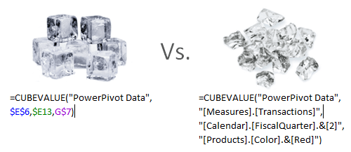
Ice Cube Method (cell references)

The ice cube method is based on referencing other cells for the member expressions in the CUBEVALUE function.  These other cells contain CUBEMEMBER functions that help determine what slice of data will be returned in your CUBEVALUE formula.

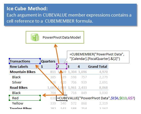
When you convert a PivotTable to formulas using the OLAP tools, you get formulas that are automatically created by Excel in the Ice Cube method.  The CUBEVALUE that is created only contains references to other cells, and those cells contain references to the members of the data model.

This is more of an indirect approach.  I call this the ice cube method because the CUBEVALUE formulas tend to be smooth and more uniform in size, but they are hard to consume without breaking them up into pieces.

Pros

The advantages are that the CUBEVALUE formula is short in length.  It is also easy to create if you already have all the CUBEMEMBER formulas setup in the worksheet.

Cons

The main problem with this type of formula is that it is difficult to understand what slice of the data is being calculated by the CUBEVALUE.  If your data model is very simple then you might be able to look at a cell that is referenced in the formula and determine what table or field it is from.  The referenced cell will only display the member name.  If you don't know what table or field that member resides in, then you have to select the referenced cell and look at the CUBEMEMBER formula to find out.

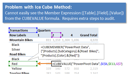
For example, the following formula references the member expression in cell $E13.
=CUBEVALUE(“PowerPivot Data”,$E$6,<strong>$E13</strong>,G$7)
Cell E13 displays the word “Red”.  To determine what Table and Field “Red” belongs to, I have to select cell E13 and read the CUBEMEMBER formula:

E13:=CUBEMEMBER(“PowerPivot Data”,{“[Products].[SubCategory].&[Road Bikes]”,”[Products].[Color].&[Red]”})

Now I can see that “Red” is a member of the “Color” field in the “Products” table.

You would then have to repeat this process for each argument in the CUBEVALUE formula to get a full understanding of what is being calculated.

This can be a bit time consuming and leads to the Crushed Ice method.

Crushed Ice Method: Full Member Expressions

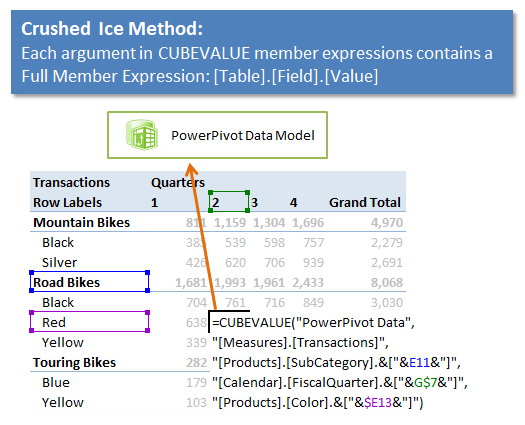
The crushed ice method refers to CUBEVALUE formulas that contain the full member expressions within the formula.  Instead of referencing other cells that contain CUBEMEMBER formulas, you can add the full string as a member expression argument in the CUBEVALUE function.

The full member expression will look like this: “[Table Name].[Field Name].[Member Name]”

And that same formula will look like the following:

=CUBEVALUE(“PowerPivot Data”,”[Measures].[Transactions]”,”[Products].[SubCategory].&[Mountain Bikes]”,”[Calendar].[FiscalQuarter].&[2]”,”[Products].[Color].&[Silver]”)

You can see that all of the member expressions are fully written out in one formula here.

As a best practice, you will probably want to change the Member Name to a cell reference.  The formula would then look like the following.

=CUBEVALUE(“PowerPivot Data”,”[Measures].[Transactions]”,”[Products].[SubCategory].&[“&$B$4&”]”,”[Calendar].[FiscalQuarter].&[“&D$3&”]”,”[Products].[Color].&[“&$B6&”]”)

This will make the formula much more reusable and allow you to copy it other cells in the worksheet to return different slices of the data.

I call this the crushed ice method because the arguments in the formula tend to be various sizes.  They are easier to consume, but sometimes more difficult to sift through.

Pros

The advantage to the crushed ice method is that you can see all the criteria that is returning the aggregated result in one place.  You do not have to jump to other cells to audit your formula.

Cons

The drawback of this method is that the formulas can get very long and difficult to read and write.  I explain some techniques for making this process easier below.

Cubed vs. Crushed?

Which method is best?  It really depends on the complexity of your report, and also how flexible you want it to be.  If you are building a dashboard with a lot of moving parts and places for user input (slicers, drop-downs, etc.) then the ice cube method might suit you better.  The crushed ice method will probably work best for static reports that don't change much month-to-month.

Whichever method you choose will depend on the layout and flexibility needs of your report.  I've found myself having a mix of both method on the same sheet.  This is probably NOT a best practice, but sometimes it is easier to just write out a CUBEVALUE formula with full member expressions versus having to create CUBEMEMBER cells in a scratch area and then referencing them.

This topic is definitely open for debate, and hopefully we can all learn from your opinion.  Leave a comment! 🙂

Convert the GETPIVOTDATA to CUBEVALUE

When you type an “=” in a cell then select a cell in a pivottable, a GETPIVOTDATA function is automatically entered in the formula.  When the source of the PivotTable is PowerPivot, the GETPIVOTDATA formula will contain the member expressions to the data model.  This is a quick way to get all the member expressions that created the slice of data for the cell you clicked on, and you can use these expressions in a CUBEVALUE function.  The GETPIVOTDATA contains some extra arguments that you will need to delete before using in the contents in the CUBEVALUE function.

There is no way (yet) to create a CUBEVALUE function by simply clicking on a cell in the PivotTable.  This would be a great feature to have in the future.

Here is a quick guide to converting the GETPIVOTDATA formula:

1. Type = in a cell then click on a cell in the pivottable. The GETPIVOTDATA formula will be created, click enter.

The GETPIVOTDATA formula contains MOST of the member expressions you will need for the CUBEVALUE formula, and it's really just a matter of copy/pasting the text to a CUBEVALUE formula.  I say MOST of the expressions because the GETPIVOTDATA formula does NOT contain the member expressions in the filters area of the pivot.  You will have to add those manually.

2. Copy all the text inside the parenthesis ( ) of the GETPIVOTDATA(“copy this stuff”).

3. In a different cell, type =CUBEVALUE(“PowerPivot Data”,

This is the start of the CUBEVALUE function.

4. Now paste the text you copied from the GETPIVOTDATA function at the end of the CUBEVALUE.

5. The GETPIVOTDATA text string contains EXTRA arguments that you need to delete.  GETPIVOTDATA contains a Field and Item argument for each expression.  You do NOT need the Field argument for CUBEVALUE, so you can delete each occurrence.  This  means you can delete every other argument in the text string, leaving only the Item arguments.  You will also leave the measures argument which is at the beginning of the string.

There is a trick that makes this delete process a bit easier.  Select the cell that contains the CUBEVALUE formula and press F2 on the keyboard to edit the formula.  You will typically see a long string of text with all the member expression arguments.

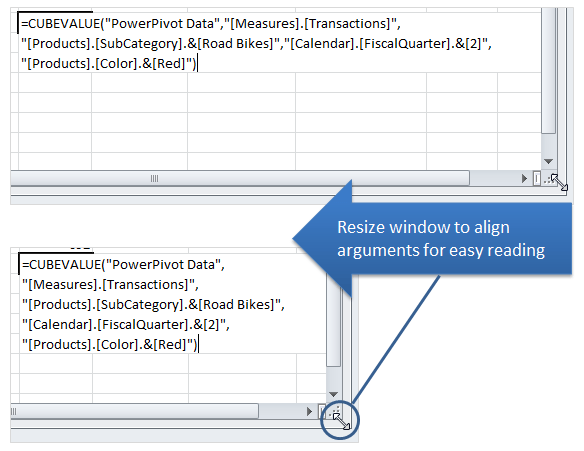
The formula will automatically wrap when it is closer to the right side of the window.  Click the Restore Down or Restore Window buttons on the Excel window, then resize the worksheet so the formula is closer to the right side of the sheet.  You will notice that as you make the window smaller, the text will continue to wrap.  You can usually line it up so that each line contains one argument.

6. Now you just need to delete every other line (argument) in the formula.  The GETPIVOTDATA function contains extra arguments that aren't required in the CUBEVALUE function.

7. Your CUBEVALUE function should now contain the full member expressions as arguments.  Press Enter to create the formula.  The results should match the original GETPIVOTDATA formula that you used as the source.

Function Arguments Window

When auditing a CUBEVALUE function using the crushed ice method you might run into the issue of not being able to see the member name of the referenced cell.  For example, cell E13 in the formula is hidden, so I don't know exactly what value is being referenced in this formula.

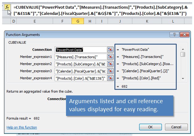
The Functions Arguments window can be used to see the value in E13.  Place the mouse cursor anywhere in the CUBEVALUE function and click the Insert Function button to the left of the formula bar.  This will open the Function Arguments window and the fully evaluated expressions will be displayed on the right side of the input boxes.  If your table and field names are long then it may be difficult to see the member name.  But this is an easy way to see all the member expressions in a list, and it will help you when auditing your formulas.

Converting between Crushed and Cubes

Here's a quick tip.  If you want to convert a formula from crushed (long) to cubed (compact), you can copy the member expressions in the CUBEVALUE formula and paste them in the CUBEMEMBER formula in a different cell.  You will then replace the original member expression in the CUBEVALUE formula with a reference to the cell that contains the CUBEMEMBER formula.

<Add screenshot>

Closing

The CUBEs are an incredibly useful functions that will allow you to create highly customized reports outside of a PivotTable.  You will probably find yourself using them often when creating dashboards and advanced models.  These tips should help save you time when working with CUBEVALUE formulas.  Please share some of your experiences and tips for working with CUBEs functions.