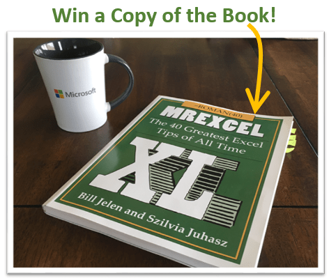
I'm giving away 4 copies of Bill Jelen's newest book, MrExcel XL: The 40 Greatest Excel Tips of All Time.
Note: The contest is now over, but checkout my review of this great book below. There is also a video at the end of the page with a tutorial on the winning tips.
My Review of this Awesome New Book
Not all Excel books are created equal. My friend Bill Jelen (aka Mr. Excel) released a new book last month titled, MrExcel XL: The 40 Greatest Excel Tips of All Time.
This is Bill's 40th Excel book, and I have to say it is probably my favorite Excel book of all time.
This book is not only packed with Excel tips and tricks, it is also very entertaining and sure to provide some laughs.
Bill has put together the 40 Greatest Excel Tips Of All Time for this book, and it is packed with awesome time saving tips and techniques. If you have ever been to one of Bill's live seminars or read one of his other 39 books, then you've probably found yourself saying, “Wow! I never knew Excel could do that!” This new book is no exception.
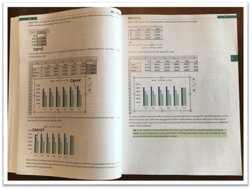
The image above is an example of one of the tutorials in this book. I'm a visual learner and really appreciate all the screenshots.
30 Additional Excel Tutorials
Szilvia Juhasz (my friend and co-host of Excel TV) co-authored this book with Bill and added 30 additional Excel tips and tricks. This was in honor of Excel's 30th birthday this year, and this section of the book is packed with some fantastic tips.
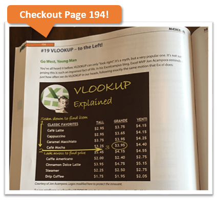
Szilvia was also kind enough to mention my name in reference to my explanation of VLOOKUP with the Starbucks menu. Checkout page 194 for that one. Thank you Szilvia! 🙂
So that's 70 Excel tips and tutorials that are clearly explained with nice screenshots and images, all on glossy pages. It's an awesome book and I have picked up some great tips from it. No matter how long you have been using Excel, there is always something new to learn.
Have You Ever Had an Excel Cocktail?
But it doesn't stop there. This book is not only a great learning reference, it is also very entertaining.
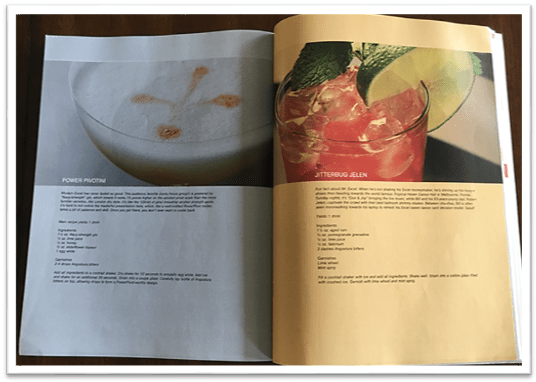
Part 3 of the book includes Szilvia's new book called, The Excel Lover's Guide to Cocktails.
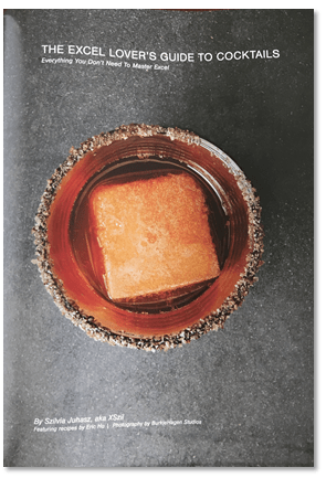
This is an Excel inspired cocktail recipe book. You will learn how to make some great drinks like the Power Pivotini (think Martini), Stacked Column Shot, Ctrl+B (think Bloody Mary), Broken Link (think Old Fashion), and many more.
The cocktail book is included as a section inside the book and contains some great pictures of each drink.
These would be a lot of fun to make for any office party, and I advise consuming after you have finished working with Excel for the day. 🙂
Get Ready to Laugh!
After you make yourself an Excel cocktail you can flip through part 4 of the book – Excel Fun.

This last section of the book includes an Excel Joke Book by Jordan Goldmeier, a collection of hilarious Excel Tweets collected by Debra Dalgleish, Excel Art by the Frankens Team, and a collection of True and Almost True Stories from Mr. Excel himself.
If you work with Excel a lot then you have experienced your fair share of ups and downs. Happy dances when things go right, and head pounding frustration when things break. This section of the book makes light of a lot of those challenges, and let's you know that you are not alone… 🙂
The inside back cover also includes the Periodic Table of Excel Keyboard Shortcuts by Mike Alexander. I love keyboard shortcuts and this is a really cool visual reference using the periodic table.
There is a ton of content packed into this 277 page book. I love to just flip through it and learn something new every time I pick it up. All the pages are glossy and you can tell that a lot of work went into the artwork and images. It's a great book to keep on your desk, or to give as a gift to your favorite Excel geek.
Win a Free Copy of the Book
To help spread the word about this awesome book, I am going to give away 4 free copies!
This will be the printed version of the the book. You can check it out here on Amazon or The Mr Excel Bookstore.
I will hold a drawing and to pick the winners at random.
I want to make it as easy as possible for you to enter the drawing. So, all you need to do is leave a comment at the bottom of this post with your favorite Excel tip.
This could be something as simple as your favorite keyboard shortcut or formula. One of my favorites is the Alt+; keyboard shortcut to select visible cells.
Add a sentence or two to describe what your shortcut or tip does, so others can learn from it. And don't worry about it being the most amazing tip ever, just something simple that saves you time.
Winners Announced!
I want to say a big THANK YOU to everyone that participated in this contest. There were over 350 unique comments, and a lot of great tips that we can all learn from.
Here are a list of the winners I picked at random. I accidentally picked 6, instead of 4, so we have two extra winners. Congratulations!
- Lynne – Ctrl+. (period) to move around selected range.
- Rajendra – Use Pivot Tables for working with numbers – Report Filter Pages
- Tom Crouch – Excel Tables and Ctrl+T
- Diane Smith – Double Clicking the Format Painter
- Matthew – F2 to Edit Text or Formula in active cell
- Debra Holcomb – Ctrl+; (semicolon) to enter today's date
Video of the 6 Winning Tips
I also put together a tutorial video of the 6 winning tips listed above.
I will be adding more videos and tutorials on the tips you posted in the future. Feel free to read through the comments below, and see how many of the tips you already know. 🙂
Thanks again!


For filling in only blank fields in a list with the same formula ……
1. Select List
2. Find & Select
3. Go to Special – Blanks
4. Fill in Formula
5. [control] + Enter
Conditional formatting is highly useful for me. It helps to quickly identify all the related cells based on my criteria, especially if the data cuts across many sheets and if there are huge data points. So the shortcut Alt+O, then D works wonders to get there quickly.
… Alt+O opens Format menu
… Then D sends you to conditional formatting rules manager windows
F2, CTRL+Enter
When you want to copy a formula in a cell to a range of adjacent cells you can select the range of cells with the active cell being the one with the formula you want, then hit F2 to go into edit mode, then hit CTRL+Enter to apply the formula to all selected cells.
The effect is similar to copy, paste special, formulas. Just easier.
There are very few things INDEX and MATCH can’t find.
I am a guy of automation. Speaking of the tools/tricks that Excel can save us time, I believe Power Query is by far the BEST tool to cut down the manual process by 99.99% in terms of data processing. Hooray!!!
Great book and awesome website!
My favorite is using conditional formatting and the if formula to highlight differences in data. In addition, using the match and index formulas to evaluate data.
When I first started using excel it was very overwhelming. Very experienced people would help me achieve an outcome using complicated formulas and I found it difficult to replicate at a later date.
The best tip I have ever received which has helped me to properly develop excel knowledge was to utilize the insert function option when completing formulas.
This function enables you to breakdown a formula and properly understand the mechanics of how it works.
I now ensure I teach other people to build their formulas this way to enable them to become more independent with excel.
Sumit Bansal’s explanation of the spell checking feature in Excel is very useful indeed, I had not been aware of this before.
I like managing data against Oracle database. Nice mix and solid 🙂
Using INDEX MATCH for looking up values in other datasets. The flexibility INDEX provides over VLOOKUP or OFFSET is the key.
My favourite shortcuts are CRL Y and CRL Z, redo and undo the last action.
My Fav tip is to use Power Query it’s awesome especially double arrows on csv files I love it
Dale
If you want to sort data in alphabetical order, you might come across cells that contain “blank” spaces in the beginning of the text string. This could be a typing error you or your data source person may have created. “Blank” spaces are considered as characters in Excel, and they have precedence over any letter. So sorting your data without “cleaning” it first would not be a good idea. You must get rid of those unnecessary “blank” spaces. Chances of having entered those spaces increases as the number of cells increases. There’s a quick way to do this “cleaning” rather than doing it manually, cell by cell, and that is by using a formula. Here’s how to do it: say you have a list of full names in column A. Call your column (cell A1) as “Clients Names”. Now insert a new column next to your list of customers. Name it the same as you did before. Now in cell B2 enter this formula =TRIM(A2)
Drag it down to reach your last row in your list and all the spaces will be automatically removed.
Then convert your formulas to values and get rid of your uncleaned data or column A. Now column B has become column A, but it is cleaned.
Now you can sort your data safely and correctly.
Bit long, but a nice time saver: In a filter list, it applies a filter to whatever cell you have chosen.
“Shfit + F10, E, V”
Ctrl + G (or F5) (both get you to “GoTo”)
Tab Tab Enter (gets you to “Special”)
K ( or Y)
Enter
Selects only the blank cells (K) or visible cells (Y) in the current highlighted range.
Awesome when editing data that’s been autofiltered.
The tip I use most must be the shortcut keys for paste special
Ctrl+c to copy
Then to paste, the list key, then S, then
V for values
R for formats
F for Formula
It always gets a “whoa, what did you do there?” from people.
I was going to say ctrl + ; as well but this is covered in the article 🙂
After that i think the best thing is the sheer ability of combinations of the lookup functions, not only vlookup but index/match combinations, offset functions, array lookups etc. Done well, these can mean you can build interactivity into the workbook and update analysis tables etc at such speed that co-workers think you’re a work demon!
Being able to automatically return different values and save so much time that would have been spent copy/pasting or manually updating is really great.
I love Excel tables. I think tables are underutilized.
CTRL+Z is Undo. NOTHING gets better than that.
Using Ctrl+` to see every formula used in the spreadshhet. It is the perfect tool when you inherit someone else’s work and dont know the underlying rules. When I discoverd this it was one of those “where have you been all my life” moments.
Vlookup the best thing that has ever come to excel. So simple to use and save time.
The best tip I can give is to read all the emails from Jon at Excel Campus and practice the tips given in his emails. This way you learn a hell of a lot great tips and excel in general.
Many Thanks
Terry
My favorite Excel tip is this formula used to count unique values in a range: =SUMPRODUCT((Range””)/COUNTIF(Range,Range&””))
Hello , Jon. My favorite are Keyboard Shortcuts, Data Manipulation.
THIS IS A MUST MASTER
Transfers to Many other applications
// CTRL + C COPY
// CTRL + V PASTE
// CTRL + X CUT
// CTRL + Z UNDO
// CTRL + Y REDO
// CTRL + F Find
and thank you for all yours excellent videos.
“Format as Table” combined with filters makes working with large data sets much easier. Using the Clear Filter button to quickly reset all of the filters is a huge time saver. Thanks!
The #1 rule in Excel is: never ever merge cells
The #2 rule in Excel is: if you must merge cells, refer to Rule #1
Merging cells renders your data useless for many advanced functions. Don’t do it. Instead select the cells & use Format Cells > Alignment > Horizontal > Center Across Selection (wrap if necessary or use Alt-Enter to put a hard return in your cells)
So true!!!
Alt = , so handy to add up the total in the range for me.
I love VLOOKUP and SUM functions to sum values from multiple columns using the power of Array CTRL+ SHIFT+ENTER to achieve the result.
{=SUM(VLOOKUP(Lookup_Value,Table_Array,{Col 1, Col 2, Col 3},False))}
This is awesome!
Ctrl – Shift – *
in order to select all cells of my database
My favourite (as in most used) keyboard shortcuts are very basic, but I use them repeatedly throughout the day to move around my worksheets. I am always surprised when I see people who have been using Excel for several years manually scrolling through thousands of rows or columns of Excel data using the mouse. If I am teaching someone how to use Excel, I alsways make sure that they know these basic shortcuts.
Ctrl+Page Down Instantly moves you to the bottom of a column of data.
Ctrl+Page Up Instantly moves you to the top of a column of data.
Ctrl+Right Arrow Instantly moves you to the right-most end of a row of data.
Ctrl+Left Arrow Instantly moves you to the left-most end of a row of data.
Ctrl+Home Instantly moves you from anywhere in the worksheet to cell A1.
If the Shift key is also pressed when using these shortcuts, then all of the data between your starting and ending position is also selected.
These shortcuts work best if all of the data in the respective row or column is contiguous, ie their are no blank cells between your starting and ending positions. If there are any blank cells, keeping these buttons pressed will allow you to move through the blank cells to you end point; it will take a bit longer but it is usually still much faster than manual scrolling with a mouse.
Give Excel boundaries! By selecting a range of cells first, Excel will create a loop to where it will only navigate through the cells contained within the range. Below I have numbered out how Excel will tab through various highlighted ranges. Note that they are numbered as if you were using the Tab key. If you were to highlight the same boundaries and use the Enter key, you would be moving north to south first and then one column to the right.
offset function is very useful when creating financial model to do analysis.
Many people already mentioned INDEX and MATCH. Another useful trick for me is F4 to repeat the last action in other cells/ranges.
ctrl-., saves time when pasting!
I love the Alt+D+E shortcut to de-segregate/segregate data from non excel files in respective columns. It is very useful all the time !
To enter current date in a cell, just press “CTRL + ; “
Pivot Table is the best … I enjoy playing with numbers so with Pivot Table its easy to make data as per my wish…
A simple tip is to use VERY simple numbers or text to generate a formula. Single digits, whole integers, and three letter texts to test and massage a formula. Then when the formula works as well as you do the easy calculation in your head, you apply to actual complicated data. Leaving the simple model intact somewhere on the worksheet for future reference.
Best tip is to visit the classy Excel websites like this one; to glean so much knowledge for so little $! Support these folks as much as you can and appreciate what we get for free.
Excellent Book!
Excellent Book!
My favorite is using conditional formatting.
F7 to spell check in Excel
Ctrl+Shift+L to invoke filter in excel (It’s a Toggle)
Use Power query to un-pivot your data set
My tip is using named ranges. Named ranges makes formulas so much easier to build and understand. Naming entire rows or columns and then using that within your formulas is really cool.
Ctrl+; is the very useful key I use every day for automatically entering the dates.
I like being able copy a cell down a column by dragging a corner down.
I have several but probably the most useful is today’s date: ctrl + ; (current time is ctrl + shift + : )
The best tip I recently was made aware of is probably the simplest. Just hit ALT on the screen you are working on and you immediately have access to various Keyboard Shortcuts!
Select visible cells (ALT+;)
Useful if you have grouped rows/columns and want to:
– Copy only the cells you are looking at to another location
– Delete specific rows without the risk of deleting hidden or grouped rows.
I often want to copy and paste borders only, and since that option isn’t native to excel I created a function that works with Ctrl+Shift+C, and Ctrl+Shift+V to do just that. See code below
Option Explicit
Private myBordersRange As Range
Sub GetBorderSourceRange()
‘Use Ctrl+Shift+C to assign source range for borders to variable “myBordersRange”.
‘Use together with “PasteBorders” macro, activated by Ctrl+Shift+V.
Set myBordersRange = Selection
End Sub
Sub PasteBorders()
‘Can only be run after “GetBorderSourceRange” code has run.
‘Activate by Ctrl+Shift+V as many times as required.
Dim myRangeP As Range
Dim i As Integer
Set myRangeP = Selection
Set myRangeP = myRangeP.Resize(myBordersRange.Rows.Count, myBordersRange.Columns.Count)
For i = 1 To myBordersRange.Count
myRangeP(i).Borders(xlEdgeLeft).LineStyle = myBordersRange(i).Borders(xlEdgeLeft).LineStyle
myRangeP(i).Borders(xlEdgeTop).LineStyle = myBordersRange(i).Borders(xlEdgeTop).LineStyle
myRangeP(i).Borders(xlEdgeBottom).LineStyle = myBordersRange(i).Borders(xlEdgeBottom).LineStyle
myRangeP(i).Borders(xlEdgeRight).LineStyle = myBordersRange(i).Borders(xlEdgeRight).LineStyle
myRangeP(i).Borders(xlEdgeLeft).Weight = myBordersRange(i).Borders(xlEdgeLeft).Weight
myRangeP(i).Borders(xlEdgeTop).Weight = myBordersRange(i).Borders(xlEdgeTop).Weight
myRangeP(i).Borders(xlEdgeBottom).Weight = myBordersRange(i).Borders(xlEdgeBottom).Weight
myRangeP(i).Borders(xlEdgeRight).Weight = myBordersRange(i).Borders(xlEdgeRight).Weight
myRangeP(i).Borders(xlEdgeLeft).Color = myBordersRange(i).Borders(xlEdgeLeft).Color
myRangeP(i).Borders(xlEdgeTop).Color = myBordersRange(i).Borders(xlEdgeTop).Color
myRangeP(i).Borders(xlEdgeBottom).Color = myBordersRange(i).Borders(xlEdgeBottom).Color
myRangeP(i).Borders(xlEdgeRight).Color = myBordersRange(i).Borders(xlEdgeRight).Color
Next i
End Sub
Hi ,
F5 – Go to Special ,
This is an awesome feature