The SUBTOTAL Metrics Macro – Create a Summary Table of All Function Types

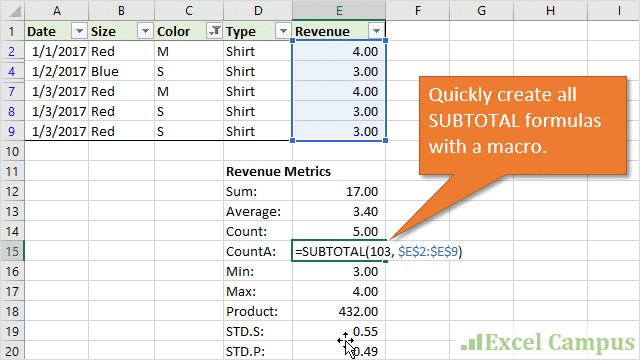
Bottom line: The SUBTOTAL Metrics Macro creates a summary table with SUBTOTAL formulas for each calculation type in the SUBTOTAL function.

Skill level: Intermediate

The SUBTOTAL Metrics Macro

During one of the VBA webinars I ran last week, Michelle had a question about creating SUBTOTAL formulas with a macro.  This gave me an idea for writing a macro to create the SUBTOTAL formulas for each calculation type.  The macro creates a summary table that includes each calculation type in the SUBTOTAL function for a specified range.

Checkout my post on an explanation of the SUBTOTAL function (including some quick tips for writing the formulas), if you are not familiar with it yet.

Here is a video clip from the live meeting where I share a macro that adds a SUBTOTAL formula to the bottom of a range, and I also show the SUBTOTAL Metrics Macro.

How the SUBTOTAL Metrics Macro Works

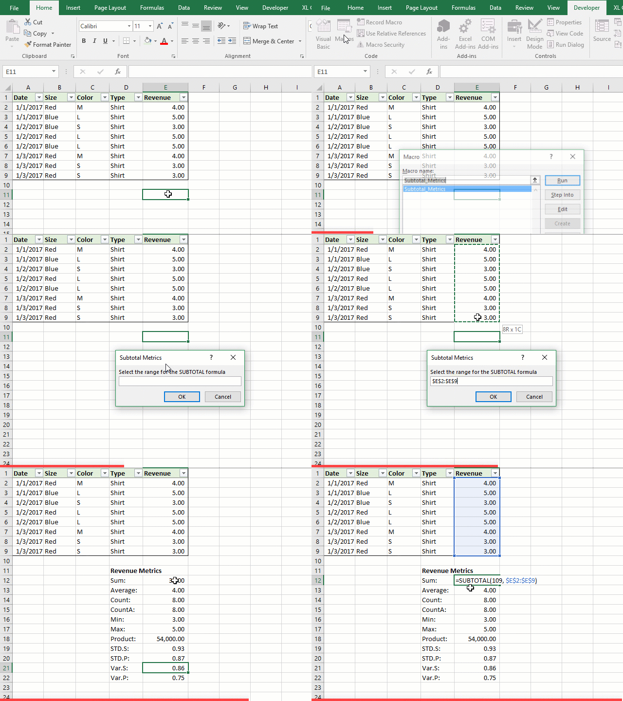
Here is a quick screencast of how the macro works:

The macro will create the SUBTOTAL formulas for each calculation type, starting in the Active Cell.  Here's how it works.

1. Select a cell where you want to place the summary table.  The output range uses 2 columns and 12 rows.
2. Run the macro from the Macros window (Developer/View > Macros), or create a ribbon button to run it.
3. If any data exists in the output range, a message box will appear asking if you want to override the existing data.
4. An input box appears and prompts you to select the ref range for the SUBTOTAL formulas.  This is the range of cells (column) that you want to perform the calculation on.
5. Press OK and the SUBTOTAL Metrics table will be created in the sheet.  A SUBTOTAL formula will be created for each of the 11 calculation types.

With just a few clicks we can quickly create a summary report for a column of data.  The formulas in the report will automatically update as we apply filters to the data range.  Again, this is very handy for tying out numbers to other reports and pivot tables.

The VBA Code & Download File

You can download the workbook that contains the code below, and add it to your Personal Macro Workbook.

Here is the VBA code for the SUBTOTAL Metrics Macro.

Sub Subtotal_Metrics()
'This macro creates formulas for all function types in
'the SUBTOTAL function. The output starts in the activecell.
'The user is prompted to select a range to include
'as the reference for the SUBTOTAL formulas.
'Author: Jon Acampora
'Source: https://www.excelcampus.com/vba/subtotal-metrics-macro/

Dim rRef As Range
Dim sFuncName() As String
Dim sFuncNum() As String
Dim
 lRow As Long
Dim lRowCnt
Dim vbAnswer As VbMsgBoxResult
Dim lFunc As Long
Dim lFuncType As Long


'The following contstant determines the Func Number series
'This can be changed to True/False to set the func_num series
'True: func_num 1-11 to include hidden rows
'False: func_num 101-111 to ignore hidden rows
Const bIncludeHidden As Boolean = False


  'Set variables - The order of the arrays can be changed
  sFuncName = Split("Sum:,Average:,Count:,CountA:,Min:,Max:,Product:,STD.S:,STD.P:,Var.S:,Var.P:", ",")
  sFuncNum = Split("9,1,2,3,5,4,6,7,8,10,11", ",")
  
  'The number of metrics listed in the table can be changed.
  'Change to 5 to only include everything up to Max.
  lRowCnt = 10
  
  
  'Check if any cells in the destination range are used and warn the user.
  If WorksheetFunction.CountA(ActiveCell.Offset(0, -1).Resize(11, 2)) > 0 Then
      vbAnswer = MsgBox("The output cells are not blank.  " _
                  & "Do you want to continue and override the existing values in range: " _
                  & ActiveCell.Offset(0, -1).Resize(9, 2).Address & "?", _
                  vbYesNo, "Subtotal Metrics")
  End If

  If bIncludeHidden Then
      lFuncType = 0
  Else
      lFuncType = 100
  End If

  'Continue running the macro if user says Yes or cells are blank.
  If vbAnswer = vbYes Or vbAnswer = 0 Then
    On Error Resume Next
      'Display an input box for the user to select the reference range for the formula.
      Set rRef = Application.InputBox( _
        Prompt:="Select the range for the SUBTOTAL formula", _
        Title:="Subtotal Metrics", Type:=8)
    On Error GoTo 0
  
    If Not rRef Is Nothing Then
        
      'Loop through all metrics in the arrays
      For lRow = 0 To lRowCnt
        lFunc = CLng(sFuncNum(lRow)) + lFuncType
        ActiveCell.Offset(lRow + 1).Formula = _
            "=SUBTOTAL(" & lFunc & ", " & rRef.AddressLocal(True, True, xlR1C1) & ")"
        ActiveCell.Offset(lRow + 1, -1).Value = sFuncName(lRow)
      Next lRow
      
      'Add title to summary table
      On Error Resume Next
        With ActiveCell.Offset(0, -1)
          .Value = rRef.Offset(-1).Resize(1, 1).Value & " Metrics"
          .Font.Bold = True
        End With
      On Error GoTo 0
      
      'Format numbers
      ActiveCell.Offset(1).Resize(lRowCnt + 1).NumberFormat = _
        rRef(1).Resize(1, 1).NumberFormat
      ActiveCell(lRowCnt + 1).Select
        
    End If
  End If

End Sub

Modifying the Macro

The macro can be modified to fit your needs.  Here are a few examples.

Exclude Unused Metrics

By default, the macro will list all 11 SUBTOTAL calculation types.  You can modify the code to exclude some of the metrics.  For example, I rarely use the Product, standard deviation, and variance calculations.

There are two arrays in the macro that contain the list of calculation type names and function numbers.  The strings that make up these arrays can be modified to include/exclude functions.  You can also change the order of how the calculations are displayed.

Here is the code for the arrays that exclude Product, STDEV, and VAR.

sFuncName = Split("Sum:,Average:,Count:,CountA:,Min:,Max:", ",")
sFuncNum = Split("9,1,2,3,5,4", ",")

Notice that I put Sum first in the list, even though it is calculation number 9.  Sum is usually the most important calculation type, and I like to have it at the top.  This is personal preference and you can modify the arrays to any order you like.  Just make sure the order of the function names and numbers match in the strings that create each array.

Include/Ignore Hidden Rows

The function number can be changed to include/ignore hidden rows. The use of 1-11 or 101-111 is determined by a Constant named bIncludeHidden. You can change the value to True to include hidden rows (1-11) or ignore hidden rows (101-111).

'True: func_num 1-11 to include hidden rows
'False: func_num 101-111 to ignore hidden rows
Const bIncludeHidden As Boolean = False

Number Formatting of the Output Range

The macro also changes the number formatting of the output range to match the number formatting of the reference range.  This can be changed in the following line of code as well.

ActiveCell.Offset(1).Resize(lRowCnt + 1).NumberFormat = _
    rRef(1).Resize(1, 1).NumberFormat

How to Use the Macro in Your Workbooks

This macro can be copied into your Personal Macro Workbook, and used on any Excel file you have open.  We can also add a custom button to the ribbon to run the macro anytime.

Checkout my free video series on the Personal Macro Workbook for more details on how to implement this.

Please leave a comment below with any questions.  Thank you! 🙂