Hide & Unhide (Filter) Columns with a Slicer or Filter Drop-down Menu

Bottom line: Have you ever wanted to use a slicer or filter to hide/unhide columns on a regular worksheet range or table?  Normally our data has to be in a pivot table to make use of the column filtering capabilities, but this simple macro allows us to hide and unhide worksheet columns with a slicer or pivot table filter.

Skill level: Advanced

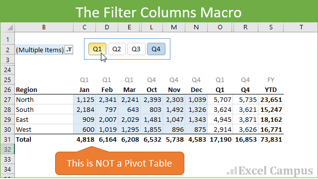
Pivot table slicers and filters are a great way to hide and unhide columns in a pivot table.  This allows us to display only relevant columns for the current time period, project, category, etc.  Hiding and unhiding columns can help reduce horizontal scrolling, which can be time-consuming on large worksheets.

However, pivot tables aren't a good solution for all applications and reports.  We cannot use pivot tables for input sheets, and reports with customized or complex column structures.

So, I wrote this macro that combines the best of both worlds.  The Filter Columns macro allows us to use a slicer or pivot table filter to hide and unhide columns on a worksheet.  This means our data does NOT need to be in a pivot table to use the functionality of a slicer or filter for columns.

Example Uses for the Column Filter Macro

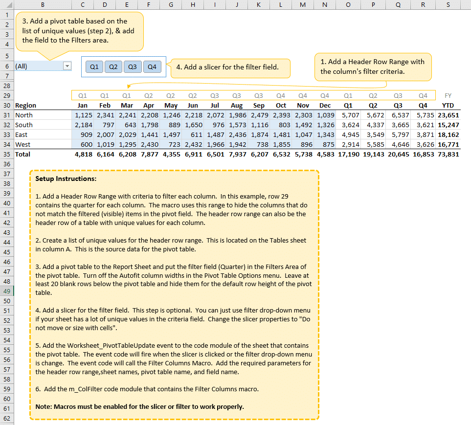
One simple example is a report with a month/quarter/year column structure, where you want to hide/unhide all month columns for a specific quarter.  This report might be a forecast/budget input sheet, or any worksheet where you would NOT use a pivot table.

The animated screencast below shows the macro in action.  The slicers are filtering (hiding/unhiding) regular worksheet columns.

Click here to view the animation in your browser.

Another example is an inventory or time allocation sheet that has a lot of columns for projects, locations, regions, etc.

How Does the Filter Columns Macro Work?

The Filter Columns macro uses a simple pivot table for the interactive controls only.  That pivot table contains one field with a list of the unique values from the header row range (column criteria) for the report.

When the user clicks a slicer item or changes the pivot's filter drop-down menu, the Worksheet_PivotTableUpdate event is fired.  The event automatically triggers a macro to run any time a user interacts with a slicer or pivot table drop-down filter menu.  This is awesome because it gives us unlimited possibilities for using slicers as interactive controls.

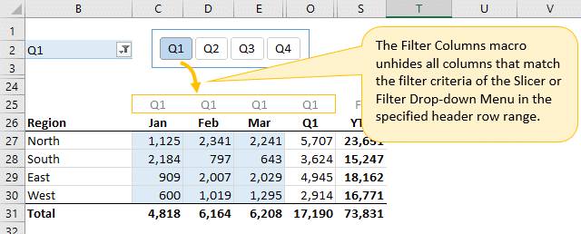
The worksheet event then calls the Filter Columns macro.  The macro loops through each cell in the header row range (column criteria) and checks if that item is selected in the slicer/filter.  If the pivot item is checked (visible), then the column is made visible (unhidden).  If the item is not checked then the column is hidden.

The end result is similar behavior to what you would expect if you filtered the columns area of a pivot table.  However, our data does NOT need to be in a pivot table.  It can be in a regular worksheet range or Excel Table.

The Filter Columns Macro Code Setup

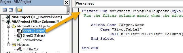
There are two macros at work here.  The first is the Worksheet_PivotTableUpdate event.  This macro runs whenever the user makes a change to the slicer or pivot table filter drop-down menu.  The PivotTableUpdate event is stored in the code module of the worksheet that contains the pivot table.

The Filter_Columns macro contains parameters/arguments that are passed through from the PivotTableUpdate event.  These parameters specify the header row range, report sheet name, pivot sheet name, pivot table name, and pivot field name.  Using parameters allows us to reuse the Filter Columns several times throughout the workbook.

Here is the code for the PivotTableUpdate event:

Private Sub Worksheet_PivotTableUpdate(ByVal Target As PivotTable)
'Run the filter columns macro when the pivot table or slicer is changed
    
    Select Case Target.Name
        Case "PivotTable1"
            Call m_FilterCol.Filter_Columns("rngQuarter", "Report", "Report", "PivotTable1", "Quarter")
    End Select
    
End Sub

Here is Filter_Columns macro code.  The macro is located in the m_FilterCol code module in the example workbook file.

Sub Filter_Columns(sHeaderRange As String, _
                    sReportSheet As String, _
                    sPivotSheet As String, _
                    sPivotName As String, _
                    sPivotField As String _
                    )

Dim c As Range
Dim rCol As Range
Dim pi As PivotItem
 
    
    'Unhide all columns
    Worksheets(sReportSheet).Range(sHeaderRange).EntireColumn.Hidden = False
    
    'Loop through each cell in the header range and compare to the selected filter item(s).
    'Hide columns that are not selected/filtered out.
    
    For Each c In Worksheets(sReportSheet).Range(sHeaderRange).Cells
        
        'Check if the pivotitem exists
        With Worksheets(sPivotSheet).PivotTables(sPivotName).PivotFields(sPivotField)
            On Error Resume Next
            Set pi = .PivotItems(c.Value)
            On Error GoTo 0
        End With
            
        'If the pivotitem exists then check if it is visible (filtered)
        If Not pi Is Nothing Then
            If pi.Visible = False Then
            
                'Add excluded items to the range to be hidden
                If rCol Is Nothing Then
                    Set rCol = c
                Else
                    Set rCol = Union(rCol, c)
                End If
            End If
        End If
        
        'Reset the pivotitem
        Set pi = Nothing
        
    Next c
    
    'Hide the columns of the range of excluded pivot items
    If Not rCol Is Nothing Then
        rCol.EntireColumn.Hidden = True
    End If
    
End Sub

How Do I Setup Filter Columns in My Workbook?

I included setup instructions in the example Excel file that you can download below.

There are about six steps to setting this up in your own workbook.  You should have knowledge of how to use and modify macros.  If you are new to macros, checkout my free 3-part video series on getting started with Macros & VBA.

I also have an article and video on how to run event based macros when the user takes an action in the workbook.

Download the Example File

The example file contains the setup instructions, macros, and the two examples I showed above.

What else can we use this for?

I feel like there are a lot of possibilities with this macro, and the use of the slicers or pivot filter drop-down menus as interactive controls.  What will you use this for?  Please leave a comment below with suggestions or questions.  Thanks!