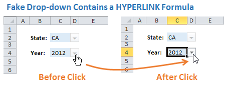
Bottom Line: The drop-down arrow (icon) for a data validation list disappears when another cell is selected. This technique will make the drop-down arrow permanently visible on the worksheet, even if the user selects a different cell.
Skill Level: Intermediate

Video: Drop-down List Arrow Always Visible
Mr Excel Podcast #1816 – Other solutions by Bill Jelen
Problem: The Drop-down List Arrows Disappear
Drop-down lists in a cell (also known as validation lists) are a great way to make your Excel model interactive. When a user selects the cell that contains a drop-down list, a small icon appears to the right of the cell. Clicking on this icon allows them to make a selection from a list.
The problem is that the drop-down icon arrow disappears when the user selects a different cell. This means the user won’t necessarily know that there is a drop-down list for them to choose from.

Solution: Create a Fake Drop-down Icon
One possible solution is to create a fake drop-down icon in the cell to the right of the cell that contains the validation list.
You can do this by placing a Wingdings 3 character in the cell to the right. Then format the cell to look like like a disabled drop-down arrow icon.

Here are the steps to create the icon:
- Select the cell to the right of the cell that contains a validation list.
- Go to the Insert tab on the ribbon, press the Symbol button.
- On the Symbol window, choose “Wingdings 3” from the Text drop-down.
- Find the symbol that looks like the down-arrow. Character code 128, or letter “q”.

- Press the Insert button, then the Close button.
- Format the cell with the following properties:
- Border Color = Grey, Border Width = Single
- Fill Color = Light Grey
- Font Color = Grey

This will create the drop-down icon in the cell and give it a disabled appearance.
When the user selects the cell to the left that contains the list, the real drop-down icon will appear.
Please see the video above for further details and instruction.
Add a Hyperlink to the Fake Drop-down
I received an awesome suggestion from the TheCric1 on the YouTube video comments about an alternative to the Input Message for the fake cell.
The suggestion was to use put a hyperlink in the fake drop-down cell that points to the cell to the left that contains the data validation.
This means when the user clicks the fake drop-down cell, the cell with the validation list will automatically be selected and the user can select from the list. The great part about this is that the user does not have to move the mouse cursor to select the cell to the left.
This article contains more info and a video on how to keep the drop-down arrow always visible.
I updated the sample file with this solution as well, and you can download it below.
It basically uses the HYPERLINK function in the fake drop-down cell. Here is the formula that you can insert into the fake drop-down cell.
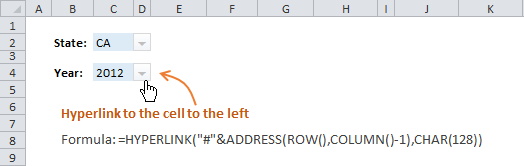
=HYPERLINK(“#”&ADDRESS(ROW(),COLUMN()-1),CHAR(128))
Choose Wingdings 3 as the font and change the formatting of the cell to give it the look of a disabled grey button.
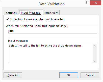
Input Message
The cell that contains the fake icon will probably fake the user at first. They are likely to click on the cell that contains the fake icon to select from the list. I’ve done it several times… 🙂

To help prevent this, I added an Input Message to the fake icon cell. When the user selects this cell, a message will appear that tells them to “select the cell to the left to activate the drop-down menu.”
To create the data validation Input Message:
- Go to the Data tab in the ribbon, then press the Data Validation button.
- Select the Input Message tab.
- Click the checkbox: “Show input message when cell is selected”.
- Type a message in the Input Message: box.
Copy & Paste to Other Cells
Once the fake icon cell is setup you can copy and paste it to other cells in your spreadsheet.
You can also download the example file and copy it directly into any of your Excel files.
Download
Download the file that I used in the video, and copy/paste the fake drop-down icon into your file.
Here is another solution based on a question from Paul in the comments. This method uses a macro and a shape that looks like the drop-down button. When the user clicks the shape, the cell to the left of it is selected and the drop-down list is opened. This uses the VBA SendKeys method which is NOT always reliable. See the notes in the file and macro code for more details.
Limitations
The biggest drawback of this technique is that the cell to the right of the validation list cell must be blank, and also be about 18 pixels wide.
If your drop-down validation lists are in an Excel Table, then you will have to insert a blank column.

Now that you know this trick, you can plan on how you will incorporate it into your model at design time.
Additional Resources
- How to Create Dependent Drop-down Lists Without Named Ranges
- How to Create Drop-down Validation Lists by Mynda Treacy at MyOnlineTrainingHub.com
- Mr Excel Podcast #1816 contains a few other creative solutions to this problem.
- Excel Tables – Learn some other benefits of using Excel Tables.
Please leave a comment below with any questions or suggestions. Thank you!


Very Creative 🙂
Thanks Sumit!
Interesting trick. This inspires me to try this trick using comment and I am quite happy with the result.
Is there a way I can put a screen shot here?
This is what I did:
Insert Comment, and Display it of course
In the comment box, leave nothing but ▼
Adust the comment box to a size of the row height and a width of a default dropdown
Move it and align it to just the next cell to the right
Format the comment box with a grey fill
Last but not least, send the comment box to back
Apply the data validation to the cell as usual.
What do you think? 🙂
That’s an interesting technique MF. I’d say the only drawback is that you would have to have the comments always visible. This might not work if there are other comments on the sheet. But still a very creative solution none the less!
Right now the only way you can post an image here is by posting a link.
Thanks! 🙂
Hi Jon,
It still works for multiple comments… although it’s quite time consuming to Show/Hide comments one by one. 😛
Cheers
Awesome Tip Jon. I will add this trick to my blog http://www.exceltoxl.com.
Thanks Abilash!
Very very clever. Great solution.
Thanks Oz! I was hoping to get a few srirachas from you. 🙂
Love the creativity in this solution. The one major drawback I see to this is most users when they see a drop down are going to click the arrow icon instead of the cell to the left. This might cause more confusion as clicking the fake drop down will not show the choices for the data validation. Does your solution address this? (I might have skipped over it accidentally)
Hi Chris,
My original solution did address this with an Input Message. However, there was a great comment the YouTube video about making the arrow icon cell a hyperlink that points to the validation cell. I updated the post with this new technique.
Thanks!
That’s a very creative workaround
[…] with drop down lists only show an arrow when selected, so Jon Acompora created a workaround, to always show an […]
Great tip, Jon.
A while back I shared a tip from Zoran for formatting the cell containing the data validation list with a custom number format which shows the wingding down arrow at the end of the text. You can see what I mean here under the bonus tip for point 1.:
http://www.myonlinetraininghub.com/excel-factor-21-hyperlink-triptych
Cheers,
Mynda
That is an awesome little formatting trick! I’ll definitely have to start using that going forward. Thanks for sharing 🙂
Very cool! Thanks for sharing Mynda!
Thank You! very much.
Thanks Phyo!
I tried using the formula you noted to create a hyperlink from the fake drop-down icon to the actual dropdown list but I couldn’t get it to work. Could you provide more detailed instruction on how to create the hyperlink between cells in the same sheet?
Like a charm. That is awesome. Thank you very much!
Thanks Zachary!
A good alternative, though it’d get time consuming if you need to do a lot of them, us by using combo boxes. In the developer tab (You might have to enable it by going to file>options>customise ribbon and selecting developer.), click on insert, and under activex Controlls, click on the combo box (second icon from the left, top row), and draw the selection box in the cell you want. You can resize it later. click on properties in the developer ribbon, and you can fill in the range under ListFillRange and the linked cell choose the cell you drew the combo box over. You can link the cell to any cell, but I find hiding the combo box over it looks better. You can change the appearance as well. When finished, if you click on the design mode icon in he developer tab, it will close and the combo box will no longer be movable or resizeable. You can click he design mode icon again to change it, and to bring the box back up to change the linked cells and range you click on properties.
Thanks for the detailed instructions Monmusu! I agree that combo boxes are another great alternative to validation lists.
This will cause the dropdown to appear right away without clicking on the arrow a second time:
Private Sub Worksheet_SelectionChange(ByVal Target As Range) On Error GoTo Err1: If Target.Cells.Count = 1 Then If Target.Validation.InCellDropdown = True Then Application.SendKeys ("%{UP}") End If End If Err1: 'do nothing End SubVery cool Dmitri. Thanks for sharing!
Hi Jon,
could you help me modified Dimitri’s cod to works when I select a shape, rather than a cell.
Regards,
Paul
Hi Paul,
Great suggestion! I just added a file to the Downloads section above that does this. It uses a shape that is an image of the drop-down arrow, and has the macro assigned to it. The macro selects the cell to the left of the shape and then uses the SendKeys method to perform the Alt+Down Arrow keyboard shortcut. You can copy/paste the image next to other cells in the workbook that contain validation. The same macro can be used for any shape in the workbook that is assigned to the macro. The macro automatically determines which shape is calling it using the Application.Caller property.
I also noted in the file that the SendKeys method is notorious for being unreliable. It should work in most situations, but it does have issues. It sometimes turns the number lock off on the user’s computer. I added a line of code in the macro to turn it back on. If this is causing issues for the user, you can delete that line of code.
I hope that helps. Thanks!
Thank you!
when Creating drop down with combo box also there is one limitation please tell me how to remove this.
when i select any option from drop down and save it –>> then again re-open this it will not show the saved value. but only blank will show there .
i am using combo box so that my drop down should be visible.
Hello,
When I used the hyperlink formula =HYPERLINK(“#”&ADDRESS(ROW(),COLUMN()-1),CHAR(128))for the fake cell, all of the wingding characters appear in the row next to the fake cell.
What am I doing wrong?
Hi LD,
The characters are appearing in the row below the formula? Do you have the text wrapped in the cell, or any other custom formatting. I’m not exactly sure what would cause that.
I am having this same issue as well. When I paste that formula into the cell with the wingdings character for the dropdown menu, it just appears in the row next to the wingdings character representing the dropdown menu arrow. Not sure how to fix this.
Hi Alex,
Can you send me your file? I’m not sure I fully understand. The cell with the wingdings character is supposed to appear in the cell to the right of the cell that contains the drop-down (cell validation). It will not appear in the same cell. Excel cannot do that.
Thanks!
Hi, I am having the same problem as above. what was the solution?
Hi John,
Can you send me your file? I’m not sure I understand this issue. [email protected]
If anyone else has this issue, you just need to click on the cell where the symbol is supposed to be and change the font back to “Wingdings 3. 🙂
Thanks for the tutorial Jon!
Thanks Leslie!
Great tip. How about this?
1) Screenshot (or snip) the real button
2) Crop it cleanly in Paintbrush, then save as a PNG format
3) Paste the picture in on the sheet wherever needed (no need to worry about column widths, fonts, etc
4) Add hyperlink to the button-picture to the input cell (so that the “real” button appears.
Hi JF,
Great suggestion! I went ahead and created the button image so anyone can right-click and save as…
The only drawback is if you had a lot cells with drop-down lists, then you would have to manually apply the link to each button. With the character and the formula you can copy/paste anywhere once you have it setup.
But for just a few drop-downs this technique will work great. Thanks again! 🙂
Hello,
Do you know how I can move the drop down button to the left side of the cell?
Thank You
Hi Kristal,
I don’t believe that is possible in Excel.
That was the my question as well. ):
Good and informative question.
Hey Jon,
I have a large workbook of data. A number of columns have data validations – lists in them which is feeding from a range on other worksheets. When I save and close out the file, the drop down feature is lost. When I scroll over the cells the drop down arrow no longer appears. The only way to see it is if I right click and select “pick from drop down list.” Is there any way to get it back to display without having to right click?
Thanks
Hi Ethan,
I’m not sure what would be causing that unless you have a macro that is deleting data validation in cells in the workbook close event.
Hi Jon,
Thanks for this solution!
I only have one follow up question:
Right now with the hyperlink formula, getting the drop down list to open requires 2 clicks. Once when you click the “inactive” drop down arrow and again when you click the real drop down arrow.
Is there a way to make it so that clicking the “inactive” arrow will automatically open the drop down list without having to click a second time?
Hi Justin,
I believe the only way to do that is by using VBA. We can use the SendKeys method in VBA to show the drop-down list when the user selects the cell. This forum post contains a macro that will do this. The SendKeys method is not always reliable and has some issues, but it should work for this simple process.
I will write up an article on this macro when I get a chance. Thanks!
Can any body please help me solving this issue regarding DV
In 2003, I was able to select arrow key of DV by clicking anywhere in cell,
but in 2010, I am forced to go to arrow key at right most part of cell.
Why this happens?
Hi Vipul,
I can’t answer the why, but that is the way it works in 2010 and later. You can also use Alt+Down Arrow to open the menu. I hope that helps
Hi Jon,
Is there a way to create a drop down menu for a cell that tells specific information instead of creating options to choose and fill in. For instance, I am creating a graph that will highlight all projects that I am working on. To give more specific information about the project I wanted users to be able to click the drop down tab on the project and specific information be viewed. Thanks in advance.
Hello,
I have the same question as you, Nadine. I’m hoping John or someone else can provide a response.
Thanks in advance.
PHS
Not sure what is the best solution out there, but I suggest using a formula / macro for this.
You mentioned you want specific information on the project to be displayed based on the user’s selection in the dropdown menu.
Let’s say this information will be displayed in Cell A10, and your dropdown is in Cell A9.
Your formula /macro (depending on how many options you have) should check the cell content of A9, and then output the corresponding text / information in Cell A10 accordingly.
Hope this helps. If you need specific instructions let me know! =) i’ll be happy to help.
-Anne-
Hey Nadine,
I don’t know the BEST solution for this, but I can suggest using a Formula / Macro to detect the Drop Down selection, and give the appropriate response in another cell.
For example, let’s say your Drop Down cell is Cell A9 and you want to give “customized” information in Cell A10.
You can insert a Macro or Formula (depending on the number of options in your Drop Down tab) in Cell A10 to check A9 content and then show the right information in Cell A10. It would be along the lines of:
– if text(A9) is ABC -> text(A10) = ABC information
– if text(A9) is DEF -> text(A10) = DEF information
If you need specific examples on the formula do let me know, I’ll be happy to help!
– Anne –
Hi Jon,
I’ve got a file with drop down list where could see it in other laptop but I could not see the drop down list at all in my laptop, any reason for that and what could be the solution?
thanks
George
Hi George,
I’m sorry, I’m not sure what would be causing that issue.
Hi, is there a way to have a drop down within another drop down? so for example, you click the drop down and have 4 options, when you hover over one option it provides an additional drop down etc. I’m trying to create a drop down where you would pick an Office building, when you hover over it, it gives you Floors, when you hover over floors you get Desk numbers to select.
Hello,
Is there any way I can click this Drop Down List Arrow using only the keyboard, and not the mouse?
Thanks
the drop down arrow is misplaced. the dropdown arrow shoulb in b4 but it is located in cell c10. it is functional but is confusing.thanks in advance.
Hi, great sharing here. After experimenting, I found a best and the most simple way that automatically select the cell and expand the drop down list at the same time with VBA macro. First create a shape with the text “q” Wingdings 3 as explained in your video. Then assign a macro.
Sub Macro1()
Range(“Q7”).Select
SendKeys “%{DOWN}”
End Sub
Hi Jon, I’m trying to insert the hyperlink into the wingdings 3 ‘q’ fake drop-down cell. How do you do it without over-riding the q ?
Hello,
I’m trying to make a data sheet and I want to have some drop down menu options but I want to have them blank until we input that line so that my pivot tables on other sheets won’t use those lines to do the pie charts until they have all the data in them. Is this possible?
Thank you, Deb
This was really helpful, thank you!
Im looking for the method to insert a black triangle in the bottom right corner of a cell, I used to hover over this triangle and an image would pop up in larger form and once I would retract the hover it would shrink back down to the triangle,l the cell size would never change when i inserted this triangle or image
Thank you author. this topic was really helpful to me and hope our community will get benefits.
thnks for sharing these tutorials.
This was really helpful. Thank you so much!
Hyperlink formula works great , but I got the Euro symbol , instead arrow , any suggestions ?Tried a few times, checked with Jon’s excel sheet .. without results.
Here we are Providing Best Template Solutionat free of Cast For all kind of Business and Examples, YOu just need to Find to your desire Topic and Download the Template
Here we are Providing Best Template Solution at free of Cast For all kind of Business and Examples, YOu just need to Find to your desire Topic and Download the Template
I took a screen shot of the drop down button and then edited it to match. Created a name for the cell with the validation list. Inserted the picture of the drop down, next to the cell and aligned it to the actual drop down button and linked to the created name.
So we have a picture that looks like the drop down and when they click it it activates the validation cell.
Thank you for the tutorials and ideas.
I found this blog very informative. If you are in search of some premium, interactive Dashboard templates, look no further than Biz Infograph. We can help you build the best presentations ever. Visit: https://www.bizinfograph.com/
Thanks in Advance
Your technique is really awesome. Actually, I was working on a Cost Statement and looking for visible drop list. But I was facing same issue as you mentioned. I was searching for the answer of the same issue and look, where I got it. Jon Acampora, thanks a lot.
Great article! Your writing style is informative and engaging, making it a pleasure to read. I especially appreciated the well-researched insights and clear explanations. Keep up the excellent work!
Check here also: https://sampletemplates.net
This is a fantastic tip! I always struggled to find the drop-down arrow in Excel, and having it always visible will really streamline my workflow. Thanks for sharing such a helpful solution!
Great post! I’ve always found it frustrating when the drop-down arrow disappears in Excel, so thanks for sharing how to keep it visible. This feature will definitely enhance my workflow. Appreciate the tips!