I've got two shortcuts for you if you'd like to filter data faster.
Video Tutorial
Watch on YouTube & Subscribe to our Channel
Downloads
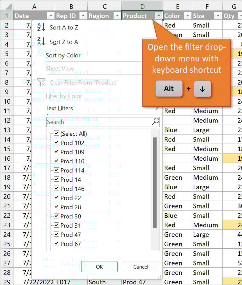
Shortcut #1: Open Filter Drop-Down Using Alt + ↓
With a cell in the header row selected (as long as you have filters applied), when you use Alt + ↓ , it will open up the filter drop-down menu.
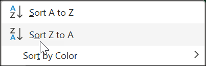
To navigate the menu using the keyboard instead of the mouse, you can use the up and down arrows or type the underlined letter to select the option you wish to use. For example, typing the letter O in the menu below will sort the column in reverse alphabetical order.
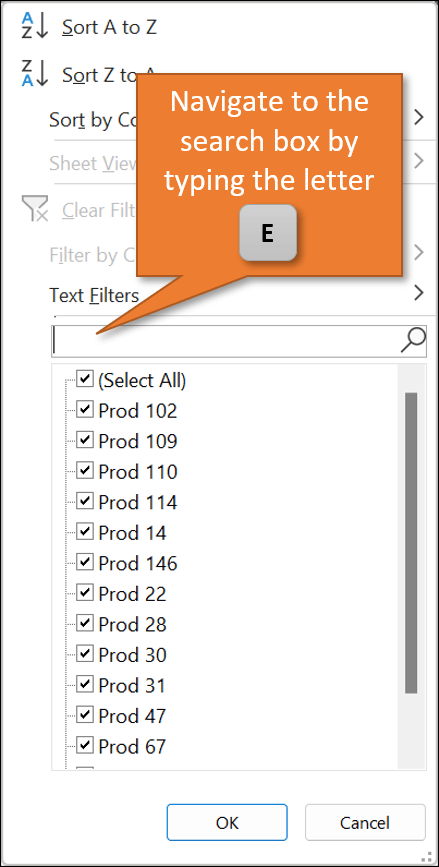
Shortcut #2: Jump to Search Using E
You can also speed up your filtering by using the search box in the drop-down menu. The keyboard shortcut to jump to the search box is the letter E.
From there, you can type whatever you are searching for and hit Enter to apply your search.
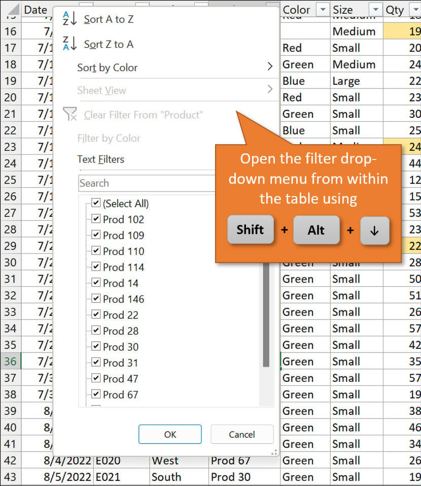
Bonus Tip: Open the Filter Drop-Down from within an Excel Table Using Shift +Alt + ↓
I mentioned above that to use the Alt + ↓ shortcut, you need to start with your header cell selected. However, if you are using Excel Tables, you can actually open the filter drop-down menu from within the table by using Shift +Alt + ↓. Your filtering will apply to the column you have selected within the table.
Check out these posts for more information about Excel filters and Excel Tables:
- Excel Filters Video Training Series
- Excel Tables Tutorial Video
- Filter Mate Add-in & Filters 101 Course
Share your filtering tips or ask a question in the comments below!


I wish we could add a Filter by Cell value button to the QAT.
You can. There is a command available, easily brought up by filtering the commands using “Commands Not in the Ribbon” (by which they mean the Ribbon MENU no matter how they pretend it’s not a menuing system) and going down to “AutoFilter”…
This gives the functionality outside Tables too, so generally useful.
It won’t apply if used on a blank cell. Blanks can be IN the range you choose, but not a single selected cell, so A1 is blank, A2:A4 are not, the range chosen can be A1:A100 (with A1 as the formally Selected cell) but choosing only A1 and no other cells, it will not engage.
More importantly, when outside a Table, it only allows a single range to be selected. You must clear that one before filtering another.
And it actually IS in the Ribbon menus, under DATA. So while this button will not clear one, only set one, that menu choice in the DATA submenu of the Ribbon menu will clear it for you. Oh, and set a new one for you in the same manner as this QAT button.
So the good news is that you can put it in the QAT, and the bad news is you don’t have to (maybe you like the QAT number key shortcuts?) as regardless of appearing in the filtered commands as not being in the menu, the Ribbon menu, it actually is in the Ribbon menu.
Lastly, the button will turn on autofilters in a Table, all, of course, as Tables do not allow autofiltering on a single column at a time, but intriguingly, while it will not turn off one it sets outside of a Table, it does also turn off Table autofiltering. So in the QAT, it would give you a toggle inside Tables, if ever of interest to you.
AutoFiltering is not something I use much, but I’ll mention there are some other oddities, but they apply to the Ribbon menu command exactly the same, so it really comes down to whether you just want mouse access by using the QAT, in which case, the Ribbon menu command is only a layer or two deep depending on how you choose to count, or if the QAT offers you other value as well (like keyboard number shortcuts).