How to Create Dependent Cascading Drop-down Lists

Bottom line: Learn how to create cascading or dependent drop-down lists (also known as cascading validation) in Excel.  This technique does NOT require named ranges.  If you don't mind using named ranges then there are a few links at the bottom of the page with solutions that will be easier to implement.

Skill level: Intermediate

Functions used: OFFSET, MATCH, COUNTA, COUNTIF, INDIRECT

Drop-Down (Data Validation) Lists

Before we dive into dependent lists, if you are unfamiliar with drop-down lists in general (also known as data-validation lists), I strongly suggest you check out my tutorial for creating drop-down lists and also this post for making drop-down lists dynamic.

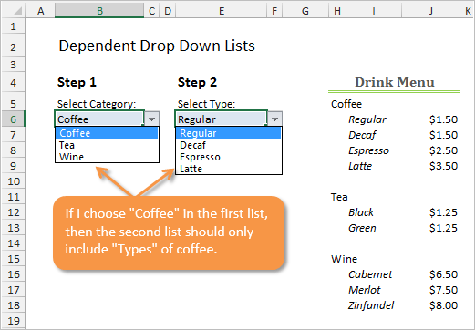
What is a Dependent Drop-down List?

Leah asked the following question, “How do I create a drop-down list where the list of choices changes when I select an item in another list?”

You can see an example of this in the screencast below.  When I select “Coffee” from the validation list in cell B4, the list in cell E4 displays different types of Coffee.

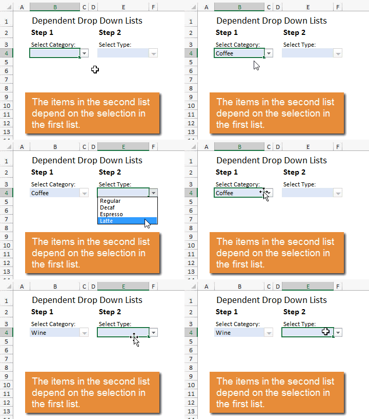
When I select “Wine” from the list in cell B4, the list in cell E4 displays different types of Wine.

These are called dependent or cascading drop-down lists because the 2nd list depends on the choice made in the first list.  This technique requires the use of the OFFSET function to create the dependencies, and it’s a great function to learn.

Step-by-Step Guide to Dependent Drop-down Lists

The rest of this article will explain how to create these dependent lists in your own workbook.  You can also download the example file to follow along, or just copy the sheets into your workbook.

Step 1: Prepare the Source Tables

Our first step is to create the source tables that we will use for the contents of the drop-down lists.

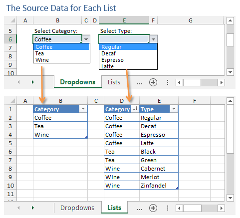
In the image above, the ‘Lists’ sheet contains the lists for each drop-down.  The list in column B contains the Category items for the parent list.  The parent list is the list where we will make the first choice.

We then use the list in columns D:F on the ‘Lists’ sheet to populate the child list with items.  The child list is the second list of choices that will be dependent on the selection in the parent list.

The first column in this table (column D) contains the Categories.  These are the exact same names that are in column B.  The second column in the table (column E) contains the different types for each category.  This is where the relationship between the Category and Type are created.

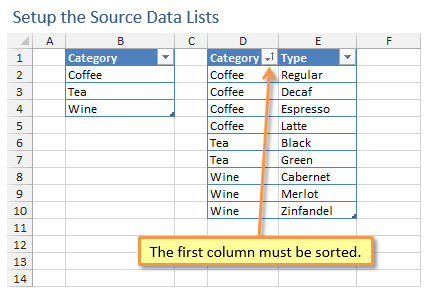
It’s also important to note that the child list needs to be sorted for this technique to work.  In the image below you can see that I sorted column D so that all the Category items are grouped together in the list.

How to Create the Lists

These lists originated from a much larger data table that contains transactional sales data.  To create the lists I needed to extract all the unique values for each list.

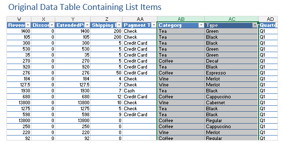
Fortunately, Excel has some great built-in tools that allow you to remove the duplicates.

One way is to use the Remove Duplicates tool that is located on the Data tab in the ribbon.

You could also create a pivot table to quickly list the unique values in the Rows area of the pivot.  Then copy/paste the results to the ‘Lists’ sheet that contains the source tables.

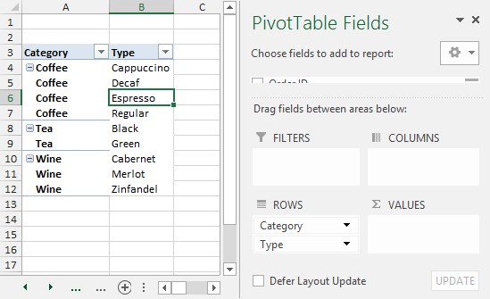
I won’t go into details on these techniques, but they will make it very fast to create and update you dependent lists.  If your lists change frequently with new items, then I would recommend the pivot table method because you can simply refresh the pivot table to generate your new list.

Step 2: Create the Parent Drop-down List

Ok, now that we have the source data lists setup we can create the drop-down lists.  We will do this with in-cell data validation lists.

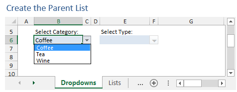
Dependent drop-down lists are not a built-in feature of Excel.  Therefore, we need to get creative with some functions and formulas to create the dynamic dependencies between the lists.

With cell B6 selected on the ‘Dropdowns’ sheet, click the Data Validation button on the Data tab of the ribbon.

The Data Validation window will appear.

1. First, choose “List” in the Allow drop-down list.
2. Then enter the OFFSET formula in the Source box (see explanation below).
3. Press OK.

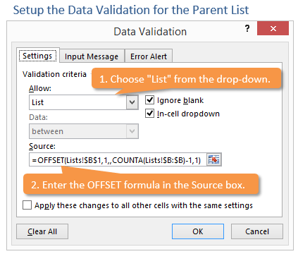
We could put the following reference in as the Source: =Lists!B2:B4

However, we want the source list to be dynamic.  Dynamic means that the list will automatically expand as we add more items to it.  We don’t want to have to change the source reference every time we add items to the list.

The OFFSET function helps create this dynamic range reference, and returns a reference to a range of cells based on the coordinates you specify.  It has the following arguments.

=OFFSET(reference, rows, columns, [height], [width])

Our Formula: =OFFSET(Lists!B1,1,0,COUNTA(Lists!B:B)-1,1)

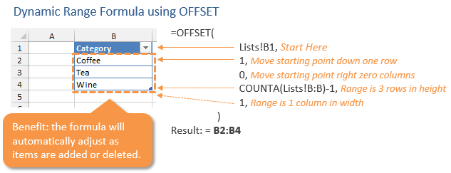
Here is a quick explanation of each argument in the formula:

• Reference – Think of this as the cell that is the starting point for the range.  In this case we are starting in cell B1 on the ‘Lists’ sheet.
• Rows – We actually want to move the starting point down to cell B2.  The rows argument allows us to specify how many rows down we should move (offset) the starting point. We put a “1” for this argument to move the starting point down to cell B2.
• Columns – This argument would move the starting point to the right a specific number of columns.  In this case we want to stay in column B, so we leave this argument blank or put 0 (zero).
• Height – This is the height of the range specified in number of rows.  In this case we are using the COUNTA function to count the number of rows that contain text in column B. =COUNTA(Lists!B:B).  This will return 4 since there are 4 rows with text in column B.  We subtract 1 because we don’t want to include the header row in our list.
• Width – This is the width of the range specified by number of columns.  Our range is only 1 column wide (column B) so we put a 1 here.

You should now have a drop-down list in cell B6 that contains all the Category items in the list on the Lists tab.

Excel Tables and the Structured Reference Alternative

If you are storing your lists in Excel Tables (which I highly recommend), then you could use the following formula instead.

=INDIRECT(“tblCategory[Category]”)

Since Table references expand and collapse automatically when rows are added/deleted, you do not need to use the OFFSET function.

Step 3: Create the Child (Dependent) Drop-down List

We now need to create the child list, which is dependent on the selection of the parent list.

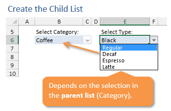
The OFFSET function can be used for this list as well.  We just need to make a few adjustments to make it dependent on the selection in the parent list.

Here is the formula for the child list:

=OFFSET(Lists!$D$1,MATCH(B6,Lists!$D:$D,0)-1,1,COUNTIF(Lists!$D:$D,B6),1)

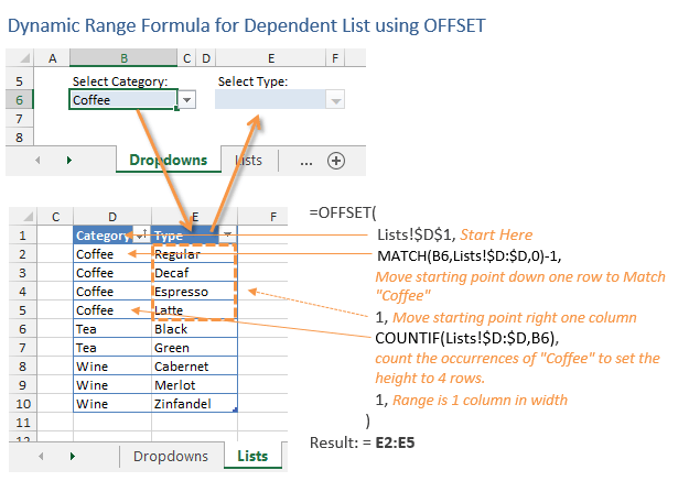
Here is an explanation of each argument in the OFFSET formula:

• Reference – Start in cell D1 on the Lists tab.  This is the top left cell of the table that lists the child items.
• Rows – Use the MATCH function to find the first row that matches the item selected in the parent list.  Cell B6 is the reference to the cell that contains the parent drop-down list.  This is basically a lookup function that returns the row number of the first matching item.  Subtract one to account for the header row.
• Columns – Specify a “1” to move one column to the right.  The formula is going to find the matching range in column D, then we have to move over one column to the right to return the range of matching values in column E.
• Height – Use the COUNTIF function to count the number of occurrences of the parent item in Cell B6, “Coffee”.  This returns a 4, which means the range will be 4 rows high.
• Width – The range is one column wide (column E).

The child drop-down list in cell E6 should now be dependent on the selection made in cell B6 on the ‘Dropdowns’ sheet (parent list).

Excel Tables and the Structured Reference Alternative

As an alternative, you could use the structured reference formulas with the Excel Table names instead of cell addresses.  The Table formula would look like the following.

=OFFSET(INDIRECT(“tblType[#Headers]”), MATCH(B11,INDIRECT(“tblType[Category]”),0), 1, COUNTIF(INDIRECT(“tblType[Category]”),B11),1)

It’s not as pretty because you have to add the INDIRECT function for each table reference.

Dependent Drop-downs WITHOUT Named Ranges

There are a few different ways to create dependent drop down lists in Excel.  The main advantage of this method is that it does NOT required the use of named ranges.

Named ranges are a great feature, but can be very confusing for some users.  Therefore, I recommend not using named ranges unless you are confident that all future users of your model will understand them.

If you don’t mind using named ranges then the following articles provide some awesome tutorials on other ways to create the drop-downs.

• Create Dependent Lists With INDEX by Roger Grovier at Contextures
• Dependent Drop Down Lists from a Sorted List by Debra Degleish at Contextrures
• Create Dependent Drop-down Lists with Conditional Data Validation  & Slicers as an Alternative to Conditional Drop Downs by Jeff Lenning at Excel University
• Great VBA & Non-VBA solutions by Jeff Weir and Roberto Mensa over at Chandoo.org

Download the Sample Workbook

You can download the sample workbook below to follow along, or simply copy the sheets into your own workbook.

How to Search a Drop-down List

Excel doesn't have a built-in option to search drop-down lists for a particular item, but I've created an add-in that gives you that option.  It's called List Search and you can access that add-in here:

Click here to download the List Search Add-in

I hope this post is useful for you! Please leave a comment below with any questions or suggestions.