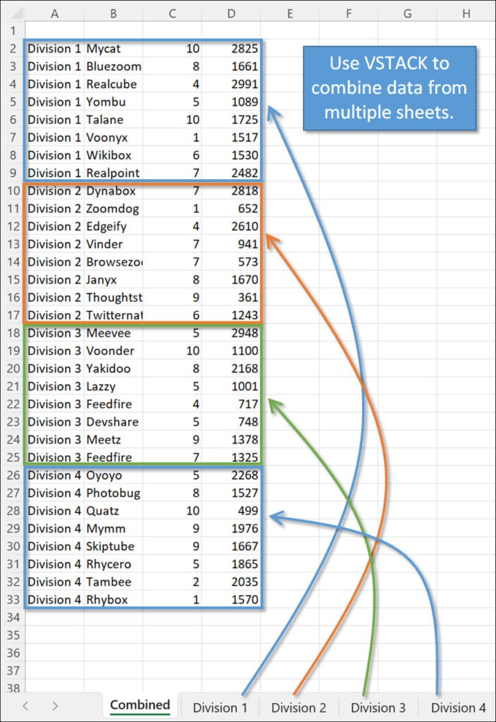
What do you do if you want to combine the data from multiple sheets into one sheet, stacking the data from each sheet?
There are many ways to stack data in Excel, but I do not recommend using Copy & Paste to do so because when data changes, you have to repeat the process all over again.
Instead, try VSTACK.
Video Tutorial
Watch on YouTube & Subscribe to our Channel
Downloads
The V stands for Vertical, and it will vertically stack all of the data from the range(s) that you specify into one sheet.
How to Write a VSTACK Formula
Using VSTACK to combine data from multiple sheets is easy!
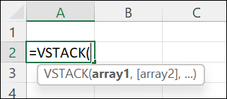
Start on a blank sheet in your workbook and type =VSTACK, then Tab into the formula. The only argument you need to specify is the array.
To pull data from multiple sheets, begin by selecting the data you want from the first sheet.
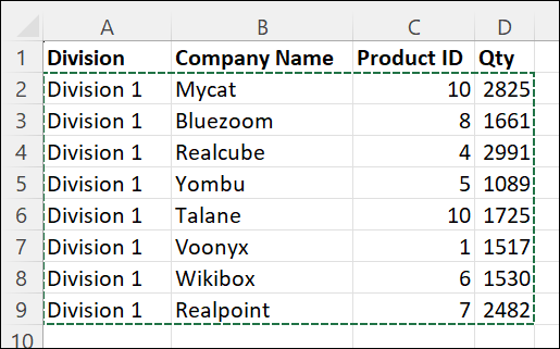
Then, while holding down Shift, select the last tab that contains data that you want to stack. In the example below, VSTACK will pull the data from Division 1 through Division 4 into the “Combined” sheet.

Hit Enter. In an instant, the data from each of the four sheets will be stacked vertically in the order of the sheets you selected.
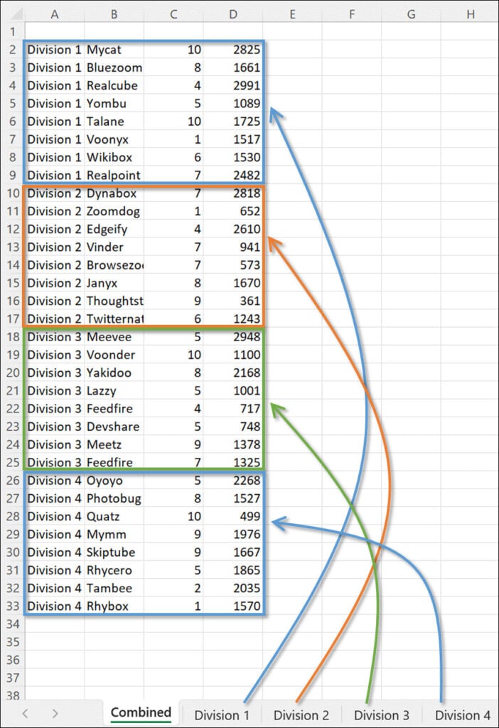
That's it! Now, when you change any entries on any of the sheets, the data will automatically change on the Combined sheet as well, thanks to the VSTACK Function,
Look for more short videos on VSTACK in the near future! In the meantime, let me know if you have questions or tips to share in the comments below.


Jon
Thanks, very useful.
I have a similar but different situation that I’m not quite sure how to handle.
The data (from an export) comes in multiple (100s) workbooks, each one with one sheet and identical fields. I need to combine all the data from those multiple workbooks into one sheet in a new workbook.
Any direction would be appreciated.
Monte
Monte,
The Power Query feature in Excel will work great for what you are describing.
If you are a member of Jon’s Elevate Excel course, it has a great course explaining it in detail, if not, just Google “combine multiple workbooks into one”.
Great question, Monte! As Daniel mentioned, Power Query is a great tool for this process.
We do have a blog post on how to combine multiple Tables with Power Query.
https://www.excelcampus.com/powerquery/power-query-combine-tables/
The process is a bit different when combining sheets from workbooks. As Daniel mentioned, we do have courses within our Elevate Excel Training Program that explain the process and setup in a lot more detail.
https://www.excelcampus.com/elevate
I hope that helps. Thanks again and have a nice weekend! 🙂
In your example I believe each worksheet had the same number of rows. What if there are varied number of rows on each sheet? Would you have to enter the comma separator for each dataset and manually select each specific array? I doubt you would reference an entire column on each sheet as I imagine it would pull all the blank rows. Would you need to format each dataset as an excel table and then do tabular column references for each array in the VSTACK formula?
In the file you can download with the examples, he uses
=FILTER(VSTACK(‘Division 1:Division 4’!A2:D12),VSTACK(‘Division 1:Division 4’!A2:A12)0)
to combine the data and remove the blank rows.
Great question, Christopher! We have an upcoming post on the formula that Kay mentioned using the FILTER function.
If you are using Excel Tables to store the data, you can also reference the table names in the formula. Although, that might be more work than the 3D reference across multiple sheets.
I hope that helps. Thanks again and have a nice weekend! 🙂
I tend to go down the Excel table route – the main advantage being the VSTACK data automatically expands and contracts as data is added to and removed from the tables.
Means you don’t have to concern yourself with the possibility of changing number of rows in the source data, as it automatically handles this.
Thanks, very useful to compare my weekly reports in pivot table .
I also insert a column in pivot table and use this formula=IF(A7=A7,”same”,”diff”)
to compare if there is difference in amount in the weekly report.
Thanks for the tip, DV! 🙂
Hi Jon,
What if you know your list is going to grow? How would you write your formula then?
Thank you,
Frank
Great question, Frank! We’ll be publishing another post that explains how to combine VSTACK with the FILTER function to filter out extra/blank rows. Stay tuned for that one.
Thanks again and have a nice weekend! 🙂
Looks so seamless!
I, too have worksheets of varying numbers of rows that I have to pull together. It should work just as well if the sheets had different numbers of rows, AND columns should it not?
I haven’t tried it yet
Thank you so much
Great question, Jesse! As I mentioned on the other comments, we have an upcoming post that will answer this question. You can use the FILTER function with VSTACK to filter out extra blank rows.
This allows you to specify a longer range, then filter out the extra rows that are blank (unused).
We’ll send out a newsletter when the new post is available.
Thanks again and have a nice weekend! 🙂
Hi john,
i am following you for more than a year. How to clone all formula and update automatically from one google sheet to work book even after replacing first google sheet and renaming second sheet with same name as first google sheet.
i have to replace AI based data sheet containing 20 FILES and i want to create summary in one page in my pc with daily update.
First day AI sheet is replaced with same name in second days and formula should not delete IN WORK BOOK when deleting first google sheet. CAN U HELP ME.
Amazing!! Every time I think I know excel, I watch one of your vids and see how much I don’t know. This works great for what I have to do.
Thank you so much
Is there any way to use a VSTACK’d table directly in a pivot table, without actually having to have the VSTACK on a sheet? I want to take a table, use a FILTER on my tblData, and use the filtered version in a Pivot. So far I’ve just made a new (hidden) sheet with the filtered VSTACK table, then used OFFSET in a named range to define “vtblData”, and then used the named range as the data source for the Pivot.
I’ve tried making a named range such as “DataRange=FILTER(VSTACK(…),…)”, but the Pivot won’t accept that. It accepts a named range “DataRange=OFFSET(…)”, but again the OFFSET requires actual cell references. Am I trying for too much?
Hi! Thank you for this, super handy!
I tried using the VSTACK formula for two dynamic worksheets, however changes are only reflected in the combined sheet from one of the two sheets. What am I doing wrong and How can I fix this?
Thank You!
needs to be dumbed down ot work for me. Thx