Bottom Line: Get explanations for common formula errors that are returned by lookup functions like VLOOKUP or INDEX MATCH.
Skill Level: Beginner
Download the Excel File
Follow along with me in the video, using the same Excel file I use. You can download it here:
Handling Formula Errors in Excel
VLOOKUP formulas can return a lot of errors, which can be both frustrating and time consuming. In this post, I'd like to show you some of the most common VlOOKUP and INDEX MATCH errors and how to deal with them.
Formula errors are typically caused by an issue within the argument(s) of the function. Formula errors always start with the pound/hashtag symbol (#).
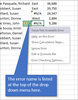
You'll notice that any cell which contains a formula error has a little green triangle in the upper left corner. In addition, there is an error button that appears next to the cell. When you click on it, you'll get a menu that gives a bit more information about the error, including the error name.
#N/A Error
The #N/A Error stands for Value Not Available. This is the most common error and it simply means that when Excel searches the specified range for a certain value, it doesn't find that value. Sometimes, that's exactly the information you need to know, but occasionally, this error is caused because of a slight mismatch that can be caused by a misspelling, extra spaces that are hard to see, or the data type of the cell.
Let's look at each of those reasons individually.
1. Typo
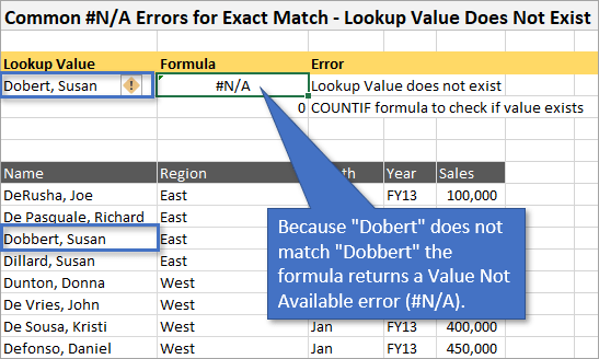
In this first example, VLOOKUP is looking to return a value for any time it finds the entry “Dobert, Susan”. But the problem is that we've misspelled the last name Dobbert, leaving out the second b. Since VLOOKUP cannot find the entry exactly as we've typed it, it returns a Value Not Available error.
The way to fix this is of course to correct the typo. Once the values match because you've fixed the error, the formula will return the correct answer that it is looking for.
Keep in mind that if the purpose of your VLOOKUP formula is not to return a value from another column, but to simply see if the value you are looking for exists, an alternative formula you can use is COUNTIF. That formula returns the number of times it finds the specified value in the range you've designated. (In other words, if there are three instances of the value you're looking for, the formula will return the number 3. If there aren't any instances of that value, you will get a 0.)
2. Number Stored as Text
The data type of your cells can also cause a mismatch between what VLOOKUP is looking for and what actually exists. So even though the values look the same (in the case below, the number we are looking for, 10001, is in our list), the problem is that Excel sees one cell as a number and the other cell as text.
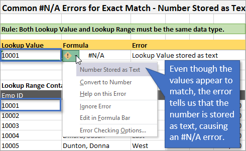
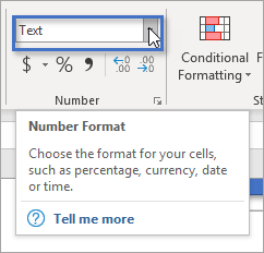
To correct the issue, you can change the data type. This can be done by choosing the second option in the menu, Convert to Number. Or it can also be done by changing the format in the Number section on the Home tab of the Ribbon.
3. Trailing Spaces
Sometimes, entries appear to match, but Excel doesn't recognize them as an exact match because one of the entries has some additional spaces trailing at the end of the value.
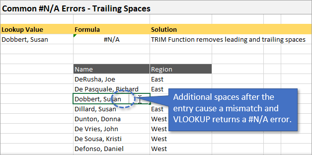
To fix the mismatch, you can manually remove the trailing spaces from the entries that have them. Or, another option is to use the TRIM function to remove any leading or trailing spaces from a range of data. Once you've trimmed them, you can either overwrite your old range with the newly trimmed range, or you can expand your VLOOKUP columns to include the newly trimmed cells.
Other VLOOKUP Formula Errors
Although #N/A is the most common error you will encounter when using VLOOKUP, there are some others as well. Three other errors that we can take a look at are #REF, #VALUE, and #NAME.
1. #REF Error
This error happens most often when columns get deleted from a sheet and that messes with the formula parameters. Usually it's an indicator that the column index is outside the lookup range. For example, the column index is set to 3, but because you deleted a column, there are only two columns left in the range.
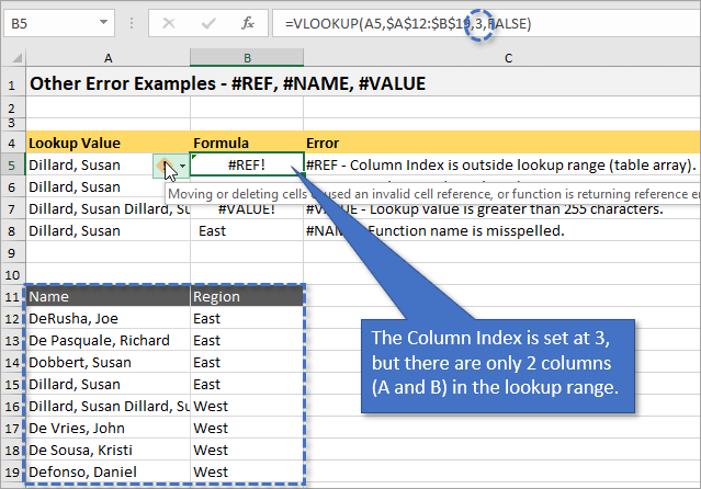
To fix the error, simply correct the column index number.
2. #VALUE Error
One reason you'll see a #VALUE error can be when you have a 0 in the column index. This sometimes happens when you use 1 and 0 instead of TRUE and FALSE at the end of your argument. To fix the problem, just correct the column index like we did for the #REF error example above.
Another reason you'll see a #VALUE error is when the lookup value contains more than 255 characters. Obviously, this is not typically something you would see, and there's really no way to correct it besides reducing the number of characters in your data, if possible.
Just a side tip: Any time you want to know how many characters are in a cell you can use the LENGTH function. Simply type =LEN and then the name of the cell in question.
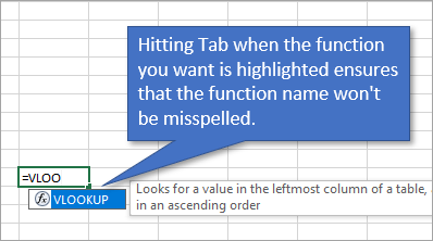
3. #NAME Error
The #NAME error occurs when you've misspelled the function name. To correct this error, just fix the spelling mistake.
You can avoid spelling errors in function names by pressing the Tab key when you start to type out the name of the function and see the one you want highlighted in the menu below your typing.
Using the IFERROR Function to Handle Formula Errors
Sometimes, the error being returned is a legitimate answer to our lookup, such as when there really isn't a lookup value in the data source, and that's just what we want to know. However, the #N/A error looks ugly on the spreadsheet.
We can return a different value for the formula error. To change the outcome so that it is blank or returns a word/phrase of our choosing, we can use the IFERROR function. The IFERROR function is a simple argument that just returns an alternate value (or a blank cell) whenever an error is found.
To use the IFERROR function, simply wrap it around the VLOOKUP formula. For example,
=VLOOKUP(A4,$A$12:$C$19,2,FALSE)
would become
=IFERROR(VLOOKUP(A4,$A$12:$C$19,2,FALSE),”ERROR”)
to return the word “ERROR” if an error is found. Of course you could make that word anything you want it to be. If you prefer that a blank cell be returned, just put nothing between the two quotation marks.
Don't Use the IFERROR Unilaterally
You might have the idea to just always wrap your lookup functions in the IFERROR function so that you don't have to see ugly errors on your spreadsheet. But I don't recommend that.
The reason is that, as we saw in several of the errors above, there is often an action that needs to be taken to fix the errors, such as correcting spelling or indexes. You definitely want to be notified of those opportunities to fix the lookup results instead of leave them as errors.
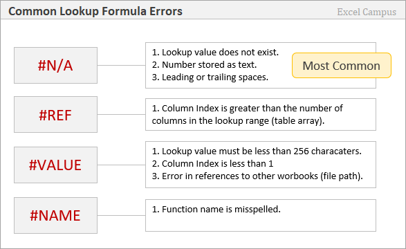
Overview of Common Lookup Errors
I've condensed all of the error reasons that we've discussed in this post into the following image. It can also be found in the practice Excel file at the top of this post or you can download the printable PDF if you prefer.
I hope this helps you to identify and fix the errors that you encounter when using lookup. Please let me know if you have any questions in the comments!


Add comment