Bottom line: Get a preview of a new app I've been working on that helps with writing lookup formulas like VLOOKUP or INDEX & MATCH.
Skill level: Intermediate
Video Tutorial
Download the Example File
You can download the sample file that contains the code below.
Update: The Create macro has been updated to handle scenarios where the lookup column is NOT the first column in the table array. See the Updates section below for details.
A Faster Way to Write Lookup Formulas
In the video above I share a preview of VLOOKUP Assistant. The goal of this app is to make it faster and easier to write lookup formulas.
The app is still in early stages of development. It is written with VBA macros, and you can download the file that contains the code above.
VLOOKUP Assistant currently has two main features.
Feature #1: Create Lookup Formulas
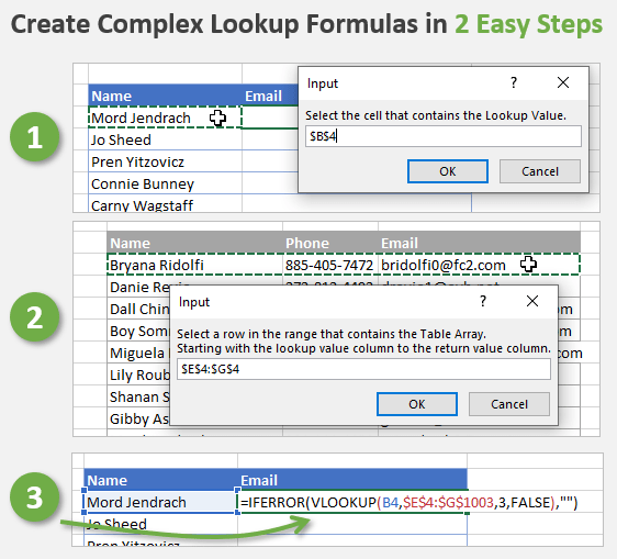
VLOOKUP Assistant will create the lookup formulas (including error handling) for you with just a few clicks. When you run the macros you will just have to specify two inputs.
The inputs are gathered using the InputBox function in VBA.
The two inputs are:
1. The lookup value
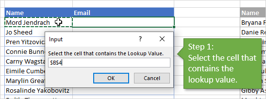
First you are prompted to select the cell that contains the lookup value.
2. The table array
Next you are prompted to select a row in the table array range. This is the range that contains the lookup column and return column.
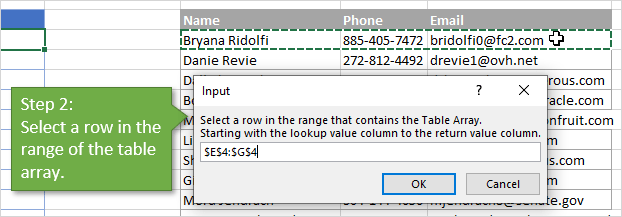
This is similar to selecting the table_array argument for VLOOKUP, but you only need to select one row in the range. VLOOKUP Assistant will automatically determine the rows to include table array and create the reference to the entire range.
This saves time from having to select thousands of rows of data, especially if you are doing that selection with the mouse instead of a keyboard shortcut.
The formula is created
The formula is then created by the macro and output to the active cell.
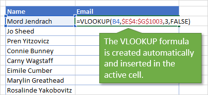
The macro determines the table_array by using the CurrentRegion property for the range that was selected in step 2. It also figures out the column index number argument based on the number of columns in the range.
The table_array range(s) are made absolute by default. This prevents the error forgetting to anchor the ranges before copying the formulas down.
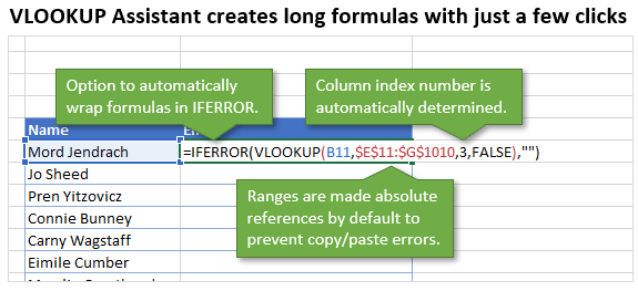
The same macro is used for both VLOOKUP and INDEX & MATCH formulas. For INDEX & MATCH, the macro just creates the lookup column and return column arguments by creating references to the first and last columns in the table_array range.

The macro also has variants that add an IFERROR wrapper around the lookup formula.
This means you can create complex lookup formulas in just a few clicks.
Feature #2: Convert Lookup Formulas
The second feature is converting lookup formulas to use other functions. The app currently converts VLOOKUP formulas to use INDEX & MATCH instead.
INDEX & MATCH does have some advantages over VLOOKUP. Mainly inserting and deleting columns without worrying about errors, and doing lookups to the left. We have a separate post coming soon with more details.
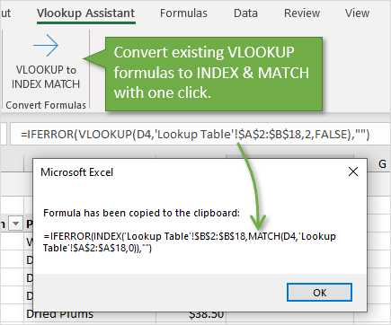
So, VLOOKUP Assistant will make this conversion with the click of a button.
- You simply select a cell that contains a VLOOKUP formula and run the macro.
- Then run the macro which extracts the range references in the VLOOKUP arguments, and uses them to create an INDEX & MATCH formula.
- The new formula is displayed in a message box, and also copied to the clipboard. You can then paste it to the active cell.
The copy to clipboard is used to retain the Undo History. If the macro were to input the formula directly then you would not be able to undo, and potentially lose the previous VLOOKUP formula that was there before.
We can also add code to paste the new formula into the active cell. That part is manual for now.
Who is it for?
I believe this tool will be useful for a few different types of users.
Frequent users
If you are someone that writes lookup formulas everyday, then you know how time consuming they can be to write. VLOOKUP Assistant will allow you to create formulas quickly.
You can also use keyboard shortcuts to run the macros and select the ranges. Everything can be done without the mouse, if that's your style. 🙂
Occasional users
If you don't write lookup formulas often, then it can also be challenging to remember all the function arguments. You might use our VLOOKUP Guide as a cheat sheet, or do a Google search every time you need to write a lookup formula.
So, this tool will walk you through the process and write the formulas for you.
Use & Installation
The app is currently a set of macros. You can download the file above that contains the macros.
Test in the Example Workbook
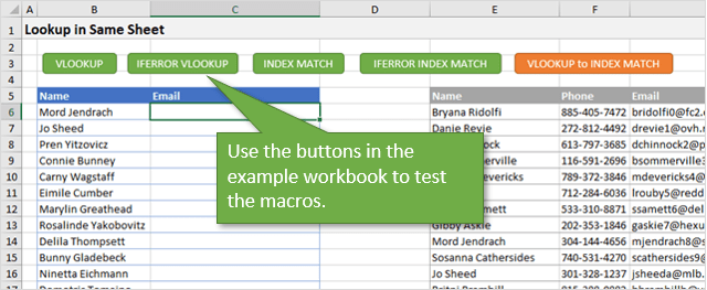
There are buttons on the sheets that will allow you to run the macros within the example workbook to test them.
Add to Your Personal Macro Workbook
You can also copy the code modules to your Personal Macro Workbook. Then create macro buttons on a custom ribbon tab to make it easy to run the macros on any open file. See video #3 on this page for instructions.
This setup will allow you to run the macros on any workbook you have open.
Here is an example of the custom Ribbon tab that I created from the Customize Ribbon menu in Excel Options.
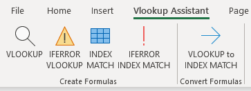
We can eventually turn this into an add-in that anyone can download and install on their computer, without having to know VBA. Similar to our free List Search Add-in.
What's next?
As I mentioned in the video, VLOOKUP Assistant is in a really early preview stage. I'm publishing it now to get your feedback.
Do you think this would be useful to you?
Do you have any suggestions for additional features?
Please leave a comment below with your answers.
Important note: The macros are only going to work in limited scenarios. They have not been heavily tested yet, so keep your expectations low. 😀
Here is a list of features I'm planning to add, and your comments below will help shape this list.
Create Formulas
- Work with Tables and create Structured Reference Formulas.
- Create lookup formulas to other workbooks. Currently only works with other sheets.
- Support for Named Ranges.
- Compatible with other language versions of Excel. Currently English only.
- Allow IFERROR to return something besides blank.
- Create Index & Match formulas that look to the left (added 8/22/19)
- Output the formula to a userform where additional options could be applied to the formula. Toggle IFERROR on/off, use COLUMNS (added 8/22/19) or MATCH in col_index_num of VLOOKUP, IFERROR return value, etc.
Convert Formulas
- Handle strings in the formula that have parentheses.
- Output the formula to a userform instead of the clipboard.
- Convert other types of formulas.
Updates & Fixes
Here is a video to explain updates & fixes I published on 8/22/2019.
Here is a list of the updates & fixes:
- Fixed bug when the lookup column was not the first column in the data range (VBA > CurrentRegion). You can now select a lookup column (table_array) that is in the middle of the data range.
- Added a new feature to use the COLUMNS function for the column index number argument in VLOOKUP formulas. This prevents errors when adding or deleting columns. See my bonus videos on VLOOKUP for more details on this technique.
- Add a new feature to create INDEX & MATCH formulas that look to the left. The process of selecting the lookup/return range in step 2 is the same. The macro just reverses the range references in the formula arguments.
So, please leave a comment to vote for any of these features or suggest other features.
Thank you! 🙂


EXCELLENT ! it will be great for index and match!
Thanks Joe! 🙂
I like it a LOT as I’m constantly using INDEX MATCH or INDEX, MATCH, MATCH. One suggestion would be to add one more macro….. INDEX, MATCH, MATCH to the options/buttons.
Great suggestion! I’ll add it to the list. Thanks Don! 🙂
This will be a time saver when working on some of my projects. Two valuable additions would be the left column lookup/index-match you noted, but also the ability to perform multi-criteria for Match would be very useful.
Thanks Bruce! The Index & Match to the Left has been added. I updated the file yesterday. I’ll add your suggestion about multiple criteria to the list. Thanks again! 🙂
I also like the fact that so far its just macro’s. I mainly use Excel at work on a company locked down laptop, so we can’t add applications.
Hi Jon,
Great tool! I think it would be a a value addition to any users toolbox. I could see this being very handy for folks who are not Excel superusers. Would there be a way to add a VBA code to name the data range.
Again I think its a great tool! Always learn something watching your videos.
Thanks Don! Great suggestion with adding the named range. It is definitely possible. I will also be adding support for Excel Tables, which essentially already have the ranges named based on Table names and structured references.
Not real helpful for me, but some of my users could be aided by it. One issue I see is that the macros assume the column to return is the last column in the range picked, but that might not be the case. I would think a third prompt to pick the column to return would be useful. For those same users, the “True” or “False” would also confuse them, so the default “False” in the macro is the safest way to go.
I was excited about your “convert VLookup to Index/Match”, but see it only handles one case at a time. I’m looking to create a macro that will convert a range of VLookups to Index/Match formulas, but haven’t gotten started yet. Your example gives me a basis to start with.
Hi Jomili
That would be quite easy to create though using Jon’s code attached.
You would merely make the user select a range and then loop through the range and instead of sending it to the clipboard, change the formulas in each cell of the range. This could even be expanded to change all in a sheet or the whole workbook. The only problem would then be that the user wouldn’t be able to undo the changes made (like with any macro). Using Jon’s example though, you could just copy down the formula if consistent in a column as well.
Renier
Hi Jomili,
Sorry, I wasn’t clear in the original video. You can select a range within a larger table range. The return column is the last column you select, NOT the last column in the range. I posted another video today in the Updates section above that explains this in more detail.
Renier makes great points about doing the conversion on multiple cells. If it is a single column of formulas that you want to convert, then those formulas are usually all the same. They might just refer to a different lookup value cell. Therefore you can just copy the formula down by double-clicking the fill handle, after the conversion.
If your data is in an Excel Table, then the autofill feature in Excel would update all the formulas in the column.
I hope that helps.
Hi Jon
I think this is excellent. The only thing I would add / change would be that the user selects the column to lookup as well. This is currently auto-selecting, but making it a 3-step process would not make it take much longer.
Great idea though. Thanks for the share!
Renier
Thanks Renier! Sorry, I didn’t explain it clearly in the original video. I just posted a video in the Updates section that explains it a little better. In the 2nd step, you select BOTH the lookup column and return column. The selection can be a smaller range within a larger data range. You do not have to select the first and last columns of the range.
However, the original file I posted didn’t work this way, so I see where the confusion came up. I have since updated the file. Check it out and let us know if you have any questions. Thanks! 🙂
Great start Jon, and I like where this is going.
Maybe one idea would be the option to run a TRIM(CLEAN) on the lookup fields without changing the cell attributes. Many imports with csv have leading and trailing spaces or special characters. (Pop up comment – Your lookup fields don’t match – do you want to apply Trim?)
Another idea may be the ability to look up values over many sheets.
ex. =INDEX(SheetList,MATCH(1,–(COUNTIF(INDIRECT(“‘”&SheetList&”‘!$A:$A”),A2)>0),0))
Thanks Again Jon
Thanks Jim! Great suggestions! I’ll add those to the list. 🙂
Jon, I cannot believe you are just giving this away. I cannot wait to “beta” test this, especially the index-match functions.
Thanks Bob! I just posted an update to the file today. There was a bug in the original one. So please test with the new file. The file has been replaced in the Downloads section. There is also a video in the Updates section that explains some new features and bug fixes.
Although I have not tried this yet, some things came to mind while reading the post. I think an add-in with these macros would be really good for users who do not use VLOOKUP regularly. It can also be helpful for learning how to use INDEX & MATCH. Could HLOOKUP be added?
A feature I would like in an add-in like this would be the ability to use multiple criteria and ranges. While SUMIFs is nice for summing values based on multiple criteria, it currently does not work if referencing a closed workbook.
Thanks Mitch! Great suggestions! I’ll add those to the list. 🙂
Very creative. Looking forward to further apps in the future. Thanks!
Thanks Joe! 🙂
Extremely helpful!! Assuming it would just be our role to assign correct column # to Vlookup as the macro wouldn’t understand what we are looking for in the table. This is amazing– thank you!!
Thanks Marci! I forgot to mention that in the video. The macro figures this out for you. No extra input is needed.
In the 2nd step you select the lookup cell/column to the return cell/column. The macro determines the column number based on your selection.
So, if you wanted to return the phone number, you would select E4:F4. Therefore, the data range can be much wider than what the lookup is looking in and returning. Your data might go from A:S, but you want to lookup a value in column D and return a value from column K. In that case you would only select a row in D:K in the 2nd step.
I’ll post an example to make this easier to understand. I hope that helps. 🙂
Hi Jon,
Extremely helpfull and very creative. Just want to discuss your description mention above. Suppose i am making a table and get the data like phobe no. and email id using vlookup from another data set but as per you description i have to select separate table array for each columns instead i want to select a single table array and just switch the col reference.
That would ease if working on big data set. Hope i am able to explain it clearly.
Thanks Lokesh! Sorry, I don’t think I explained it clearly in the first video. I posted a new video in the Updates section today that explains how to do the selection when your lookup and return ranges are in a narrower range within a larger table.
The column index number is determined by that selection. However, there currently isn’t a way to specify a smaller column index number. In the example, if you select to the Phone Number column, then the column index number will be 2. If you select to the Email column then column index will be 3.
I hope that helps.
I had the same question as to how you determine the column to return. The way you explain it there, it will always return the value from the last column of selected range?
Hi Erik,
Sorry, I wasn’t clear on that in the first video. The column index number is determined by the last column you select. Not the last column in the table. I posted another video in the Updates section today that explains that in more detail.
The original file also didn’t work this way, and I updated it yesterday to include this functionality.
Therefore, you can select a smaller range within a larger table to lookup and return columns within the table. It does NOT have to be the first and last column of the data range (table).
I hope that helps.
vlookup is a workhorse for me. As you know, vlook finds first instance. Index and match can be configured to find multiple names (for example), but it is difficult for the occasional user. A macro to search a list of [names, businesses] , find an amount [for example] and then the next instance of the same name in the list with the next instance. Difficult to say this. Built a quick sheet to demo, but can’t paste it. Thanks for what you do.
Thanks for the suggestion Cliff! I believe I understand your request. I’ll add it to the list.
The new FILTER function with Dynamic Array formulas will also make this task MUCH easier. Here is a post on those new functions.
I hope that helps.
This is great! Would it be possible to add the error handling as a separate step as well as including it as an initial setup option? When I was playing around with this, I used just VLOOKUP first but noticed down the line that there were errors. Adding error handling manually is pretty easy, but if done after the formula is in place and using an input box, that would be super slick!
Thanks Elizabeth! That is a great suggestion! Yes, it is definitely possible. Are you saying the input box would prompt you for the value_if_error value?
I’ll add it to the list for future updates.
Do you have something that would help when there is a “close” match, meaning I get list where the person’s name in a list might have their nickname, whereas the payroll listing will have their formal name? Examples: Bill Smith versus William Smith, or Connie Bunney versus Constance Bunney. Almost always, they are one and the same, but I end up reviewing manually and looking for a way to flag the “close” ones, versus the ones that absolutely do not match.
Hi Wally,
Great question! That’s typically referred to as a fuzzy lookup. Microsoft does have an add-in that helps with that. Here is a link to the download page.
I don’t have much experience with it, so I can’t comment on how well it will work for your scenario.
I hope that helps.
I love this, but will it work on Mac? Office 365?
Hi Diane,
Yes, it should work on the desktop version of Excel for Mac (Office 365). I have not tested it yet, but feel free to leave a comment here if you have any issues with it. Thanks!
great stuff, definitely have a use for this. Thanks again!
To improve the current version of your macros:
The message box saying “Select the cells that contains the Table Array.” can be made more accurate by saying something like
“Select some cells in one row of the Lookup Table Array, ending with the column with the data that you wish to have returned.”
For the Index Match application:
There should be 3 message boxes.
The first would say (as it does now) “Select the cell that contains the Lookup Value.”
But there should be two “OK” buttons, one for “OK Unlocked col (no $)” and the other “OK Locked col ($).”
The second message box would be “Select one cell in the Lookup Table Array in the column with the values you wish to search.”
The third message box would be “Select one cell in the Lookup Table Array in the column you with the values you wish to return.”
(this will allow searches to left and right from any starting column.)
This third box could have three OK buttons: “OK-Exact Match”,”OK = lookup_value.”
Since Exact Match is used the most by far, the “OK-Exact Match” button could be very large and the other two OK buttons very small.
Thanks for the suggestions, Dan! I posted an update today with a more descriptive input box for step two.
The update also fixes a bug that was only allowing you to create formulas that were looking up the first column in the table and returning the last column. That was NOT the intended purpose, and I’ve fixed it. You can now select a range within a larger table for the lookup and return.
I also added the ability to do Index & Match to the Left. This still just requires you to select a single range in step 2. The “to Left” option is specified when you run the macro, and then it just reverses the range refs within the formula. I explain it in more detail in the video in the Updates section on this page.
I believe this process can remain a two step process for the vast majority of cases for writing a lookup formula.
I hope that helps. Please let us know if you have any questions or suggestions. Thanks again! 🙂
This looks like it can save some time, very well done Jon!
Thanks Josh! 🙂
Very cool. I created a similar macro last year using some of the same methods. I also incorporated TRIM, SUBSTITUTE, and CHAR into my formulas to remove any “hidden” spaces that may exist, as well as coding to pull the formula down to the end of the lookup value’s column, though I haven’t perfected this portion just yet, as my lookup formulas always end up going a few rows beyond my lookup value’s column. You could program that step into the app to eliminate the manual click-and-fill action. Looking forward to seeing this app evolve, as I am sure it will save A LOT of time for people. Nice work!
Hi Jon,
So, it’s the same as =VLOOKUP(B11,Sheet2!$E$11:$K$11, COLUMNS(E10:G10),0). Where E10:G10 represent the header row of your lookup table and G10 represents the lookup value column?
Thanks,
Colin
Hi Colin,
This is different from Luke’s comment. His comment is about copying down rows.
I just updated the macro with a new feature to add the COLUMNS function for the column index number. There is a video in the Updates section with more info.
I hope that helps. Thanks! 🙂
Thanks Luke! Yes, the macro could do the fill down automatically. You would lose the undo history though. In the final product, I will probably implement a feature that allows you to use the copy to clipboard and paste the formula in the active cell, to keep the undo history.
One easy solution for this is to use Excel Tables. The formula will automatically be copied down when it is inserted or copy/pasted into the cell.
Here is an article that explains how to find the last used row with VBA, which might help with your macro.
Thanks!
Jon- Great tool to be used. It will be awesome, if you do it as add-in to use in any project. I’m a heavy user of Vlookup, Index & Match and can you add a Hlookup as well…..
Thanks Will! Yes, we will turn this into an add-in. Thanks for the vote!
I’ll put Hlookup on the list for future features. 🙂
Will your app run on a Mac?
Hi Charlie,
Yes, it should run on the Mac version of Excel. I haven’t tested it yet but will do that later today. Of course, feel free to try it out and leave a comment here if you have any issues. Thanks!
Jon, I tend to use data modeling instead of vlookups, but I sent your email to my son who was very excited.
What do you mean by “use data modeling instead of…”?
Are you referring to Power Query?
Hi Renier,
I believe Kris is referring to Power Pivot. The term Data Model and Power Pivot really mean the same thing.
Here is an article that explains How to use Power Pivot Instead of VLOOKUP.
I hope that helps.
Jon, this is amazing, huge time saver, I love it. Looking forward to the add-in.
Thanks so much Lonnie! 🙂
Great idea. But…
You never ask for which column has the value to be returned. In a spreadsheet with many columns with multiple data types, how do you determine which value to return. I’d add an third input box asking for the column to be returned.
Hi Andy,
Sorry, I forgot to mention this in the video. The column to be returned is the last column you select in the 2nd step. You do not have to select an entire row in the table array. Instead, the first column you select is the lookup column and the last column in the return column. So you can just select a few columns in the data range, not the entire table.
The only place this doesn’t work is if you are doing an INDEX MATCH to look to the left. I’m planning to add another option that handles that.
I hope that makes sense. I’ll post another video that explains that.
Hi Andy,
Just wanted to follow-up and mention that the original macro was not working the way I explained in my comment to you. I have since updated the file and it will now work when you select a range within a larger table.
Looks impressive to me.
Great work, Jon. Looking forward to the final add-in.
Thank you Jon.
Anything that saves time is worth its weight in gold these days, and as Excel is a time saver, condensing time expended even more has to be of merit. I will investigate this as although I am no longer in the world of work, I use Excel almost every day in my role as a charity volunteer.
When I first saw Index Match, I thought it would nest the Match function with the vlookup for a 3 dimensional formula:
=VLOOKUP(B6,$E$6:$G$1005,MATCH($C$5,$E$5:$G$5,0),FALSE)
Since this is all about saving time, would it make sense to use the Columns function for the 3rd argument in the vlookup?
=VLOOKUP(B6,$E$6:$G$1005,COLUMNS($E$5:$G$5),FALSE) instead of
=VLOOKUP(B6,$E$6:$G$1005,3,FALSE)
Hi Stephen,
I posted an update today that has a feature for adding the COLUMNS function for the column index number argument. There is a video in the Update section that explains more.
I’ll add the MATCH function in VLOOKUP to the list for future updates. Thanks! 🙂
I really like it. Using Excel VBA to make development easier. I like it. Thumbs-up
Thanks Michael! 🙂
I know how to use Vlookup and Index/Match (more or less), but I am having a hard time using Index/Match as I use VLookup for just about everything, and I feel like Index/Match is more complicated and is not that much different. Perhaps I need to see a real complex situation where Index/Match would work and VLookup would not. For example is there a way to do a Right to Left lookup instead of a Left to Right? Would that be a benefit of Index and Match?
Hi Srini,
Great question! I’ll be posting an article and video in the coming weeks that explains the benefits of INDEX & MATCH over VLOOKUP.
There are a few main reasons including the one you mentioned with returning a column to the left. The other is preventing errors when you add or delete columns in the table array.
I hope that helps.
Jon,
Thanks for this code. I tried using this in a file that I have manually added many IndexMatch formulas to and it does not reference the correct data. The original formula was ‘=INDEX($BN$2:$BN$102,MATCH(J2,$BM$2:$BM$102,0)) which was correct. When I tried replacing it using your code, I got ‘=IFERROR(INDEX($C$2:$C$106,MATCH(J2,$B$2:$B$106,0)),””). The formula is in cell N2 and my lookup value was in column J2 (four columns to the left) and my lookup array table was BM2:BN102. I was trying to return the value from column BN. Note that column J is 106 rows long but my lookup array (BM&BN) is only 102 rows long. For some reason your formula shows column C as the index array although I have selected cell BM2:BN2 and it also shows column B as the Match lookup array . I have tried many different things but can’t get the correct result. I could send you this file if you are interested in looking further into this. I do think this would be a helpful tool when working correctly.
Hi Bud,
Thank you for reporting this. I realized that the macro was not working properly when the lookup column was NOT the first column in the data range. I just fixed the file and updated it in the Downloads section on this page. I also added functionality to do a INDEX & MATCH to the Left. There is a tab in the back of the workbook where you can test this as well.
When you get a chance, test it out with your data and let us know how it works. Thanks again and have a nice day! 🙂
Jon,
This is awesome! The only minor problem that I have is when I call the macro the actual file is opening and then I have to switch back to the file I am working on. Otherwise it works great!
Jon,
One suggestion that would make this an incredible resource; add the ability to do Index/Match array formulas for multiple criteria. Such as ‘=INDEX($CA$11:$CA$16,MATCH(1,(Y10=$BX$11:$BX$16)*(AB10=$BY$11:$BY$16),0)). Obviously cntrl+shift+enter has to used for these array fomulas. Thanks.
This is a terrific idea. I have one suggestion – what about another button to add the formula and then convert the range you copied the formula into to a value.
Thanks for the suggestion Di! We could definitely add a feature to convert to values. Similar to copy/paste values.
Awesome idea! So many people in my office get stuck doing this sort of thing, now they can use this to help them get the hang of it
Thanks Mitch! I’m happy to hear it will be useful! 🙂
What a Time Saver – Thanks Jon
Thanks David! 🙂
Dear Jon, I love this & I love you!
Why don’t you also incorporate the case of VLOOKUP with approx. match in the macro & your tutorial/app?
Thanks Sandeep! I really appreciate your support. I’ll add approx match lookups to the list for future updates.
Awesome !!!
Jon,
In the video presentation VLOOKUP formula pick the col_index_num automatically. What if we need to choose a different col_index_num? Do I add another column head in the sheet.
Thanks Eugene! I posted another video in the Updates section today that explains more about selecting the return column. Sorry, I wasn’t clear in the original video.
You can select a lookup and return column within a larger data range. The macro figures out the column index number automatically.
However, as it works right now, the column index number will be the number of columns you select in step 2. The last column you select in step 2 is the return column.
If you wanted to have a larger table array, and smaller number for the column index number, you would just need to manually change that number in the formula.
It is possible to add a step to specify a column index number, but in the vast majority of cases I think we typically specify the table array out to the return column.
I hope that helps. Please let us know if you have any questions. Thanks! 🙂
This rocks. What a timesaver. Well done.
Thanks Don! 🙂
Besides the use of Input Box & User Form, you may also consider using Form provided with Formatted Table.
Hi Jon – Once upon a time, I used to write a lot of VLOOKUP formulas. Not so much anymore, so when I do need one, I have to spend time rummaging through the attic of my brain or spend time researching when that doesn’t work.
Thanks for sharing this great time-saving tool. So then, are you planning to add similar features for HLOOKUP as well? …as the monster says in the movie “Little Shop of Horrors”, “FEED ME”! LOL
Hey Tom,
LOL! I think the phrase “if you don’t use it, you lose it” was invented exactly one month after VLOOKUP was invented. 😉
Yes, HLOOKUP has been a popular request and it’s on the list for future updates.
Thanks! 🙂
Outstanding! What a great tool to have available!
Thanks Rich! 🙂
Great idea. Looking out for the final product!
Yes I think this help would be great.
Will it work on a sheet that is not defined as a table?
Thanks Rick! Yes, the ranges in the example I showed were NOT formatted as Tables. They just looked like Tables.
I will be adding support for Tables and structured reference formulas.
Hi Jon, keep up the great work!!
I’d like to know how to copy an entire worksheet to another worksheet with one select, copy and paste.
The target worksheet contains formulas, titles, headings, formulas, bold formatting, etc. In other words it’s a form.
The source worksheet has the values located in the cells locations where the values need to go in the target worksheet.
Can I copy the entire source worksheet cell values only to the target worksheet and preserve the target worksheet form/titles/formulas?
I like it.
It would be a time saver and will eliminate keyboard errors when typing in these long formulas and then having to find your key stroke errors.
Would definitely use it.
I have taught my own Excel classes and tell my classes when I get to VLOOKUP that I use this formula in some workbooks 40,000 time more than the SUM function.
Question, how do you determine the third argument “column” in the VLOOKUP function? I know it is in code, just want short overview.
Most students struggle with the fourth argument in VLOOKUP functions. To them If you want an exact match the true seems to them like a better identifier for an exact match than false.
Thanks Henry! Great question! The column index number is determined by the number of columns that are selected in the second step.
That selection will be from the lookup column to the return column. It does NOT have to be the entire width of the range. I posted a video in the Updates section on this page that explains it a little better.
Even though VLOOKUP or INDEX/MATCH require four arguments, there are really only two inputs needed to create the formula.
1. The lookup value
2. The lookup/return range.
The rest can be figured from those inputs. That’s the goal of VLOOKUP Assistant. To create these formulas in the fastest and easiest way possible.
I hope that helps. Please let us know if you have any questions. Thanks again and have a nice weekend! 🙂
John, Thanks for your response. I did not read your response and found looking at your code that, as you say in your response, the lookup column is always the last column in the data range.
I know that this is very new and you may have thought of this but not implement it yet.
You could lookup any column in the database if that column had the same heading as the heading in the column containing the formula. If this was so, you could determine with the MATCH function using the name of the column the formula is in, looking in the header row of lookup table to find the lookup column number.
This is great. I have a cheat sheet sticky note with the layout of INDEX/MATCH since I’ve gone to using that all the time.
One suggestion is since you do mention having the search/return data in a table array – why not enhance the macro to use the actual table name and table column headers. This way if your search/return table contracts or expands with more row data the formulas still work vs absolute values.
Thanks John! That’s a great suggestion with Tables and structured references in the formulas. It’s high on my list of feature updates. 🙂
This is a great assistant. Really helpful in taking complex formulas and making them easier to create. Nice work and I appreciate the downloadable file and all the other instructions you provide. Thanks.
Thanks David! I appreciate your support. Have a nice weekend! 🙂
Thank you, this is a great tool!!
Looks great so far. Most of the data I work with are in table format, so am looking forward to that enhancement to this future Add-In.
Like this idea alot. Any reason why you wouldn’t include the “$” in front of the ID reference for the Vlookup function –> ie =vlookup($A1,…..) ? I’m thinking theoretically if you were copying the lookup formula over, you would not want to lose the column reference to your ID column.
Also would be nice to have the option to make the vlookup column reference dynamic (maybe using the column function).