The Excel SUBTOTAL Function – Calculations on Filtered & Visible Cells Only

Bottom line: Learn how the SUBTOTAL function works in Excel to create formulas that calculate results on the visible cells of a filtered range or exclude hidden rows.

Skill level: Beginner

The SUBTOTAL Function Explained

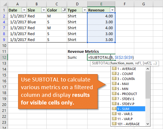
The SUBTOTAL function is a very handy function that allows us to perform different calculations on a filtered range.  The most common use is probably to find the SUM of a column that has filters applied to it.

The SUBTOTAL function will display the result of the visible cells only.  This is great for tying out numbers in a filtered column to summary reports and pivot tables.

SUBTOTAL actually gives us eleven (11) different functions to choose from.  We can use it to return the SUM of the filtered range, or any of the following calculations.

1. AVERAGE
2. COUNT
3. COUNTA
4. MAX
5. MIN
6. PRODUCT
7. STDEV.S
8. STDEV.P
9. SUM
10. VAR.S
11. VAR.P

That means we can use SUBTOTAL for any of the different calculation types listed above.  However, only ONE of the calculation types can be used in the formula to return the result to a single cell.

How to Write a SUBTOTAL Formula

The SUBTOTAL function is pretty simple.  It just has two required arguments.

Argument #1 – function_num

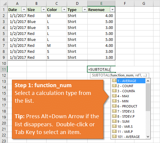
The first argument is the function number.  This allows us to specify which of the eleven calculation types we want to use, and we can select the number from the drop-down list in the formula editor.

To select an item in the list, double-click it or press the Tab key.

Quick Tip: If the drop-down list disappears, you can press Alt+Down Arrow to view it again.

You probably noticed that the calculation types are listed twice.  One set that is single digit number, and another set that stars with 101.

• The 1-11 functions will include hidden rows
• The 101-111 functions will ignore hidden rows.

Hidden rows are different from filtered rows.  Both calculation types will excluded rows that are not visible due to filtering.  However, if we were to hide additional rows in a filtered range then the 1-11 functions would still include these hidden rows in the result.  The 101-111 functions would not include the hidden rows.

So, if you only want to see the results for visible rows, regardless of how the rows are hidden, then use the 101-111 functions.

The argument is specified by typing the single number 1-11, 101-111 in formula.  When we select an item from the drop-down list, it will automatically put the number in the formula.

We can also reference a cell that contains the number of the function.  This can be used for a dynamic formula where you might want the user to select the metric from a drop-down list.

Argument #2 – ref1

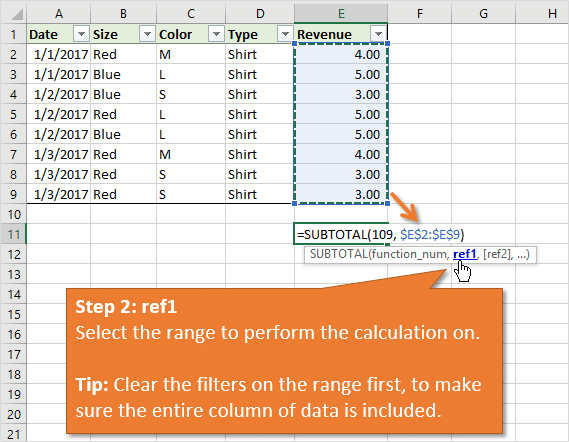
The second argument is the range (column) of cells we want to perform the calculation on.  We can simple select the range of cells or type in the range reference.

This range will typically be a single column that has filters applied to it.

Don't forget to make the column and/or row references absolute (F4 key), depending on if you are going to copy the formula down/across.

Additional ref Arguments

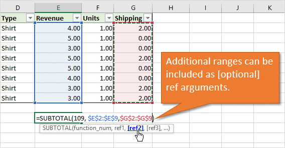
We can also add additional ranges to the formula.  We can include additional columns that are not contiguous (next to each other), by adding additional ref ranges to the formula.  These range references are separated by a comma.  We can add up to 254 additional range references.

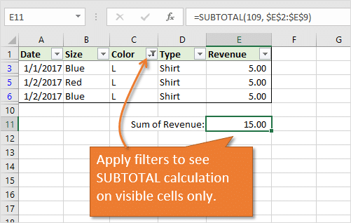
Apply Filters To See The Calculation on Visible Cells

Now that we have the SUBTOTAL function written, we can apply filters to multiple columns in the range.  The SUBTOTAL function will return the results of the visible cells only.

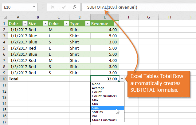
Excel Tables also use the SUBTOTAL function in the Totals Row of a Table.  You can select one of the calculation types from a in-cell drop-down menu in the Totals Row, and the SUBTOTAL function will automatically be created for you.  This is one of the many time saving benefits of using Excel Tables.

Checkout my video on a beginner's guide to Excel Tables to learn more about this awesome feature.

Bonus tip: The SUBTOTAL function can also automatically be created with the AutoSum feature when the range we are applying it to is filtered.

I also have an article and video on how to select and copy/paste the visible cells only.

The SUBTOTAL Metrics Macro

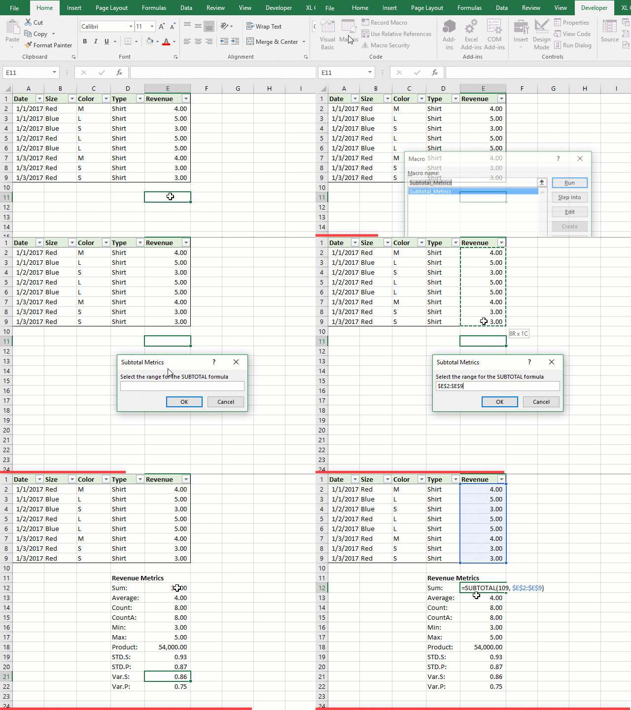
Sometimes we want to use the SUBTOTAL function to calculate more than one calculation type on a column.  For example, we might want to see the Sum, Min, Max, Count, and Average of the column for quick analysis.

Typing a SUBTOTAL formula for each calculation type can take some time.  So, I wrote a macro that creates all the formulas for us with just a few clicks.

The SUBTOTAL Metrics Macro creates a summary table on the sheet with a SUBTOTAL formula for each calculation type based on range that you specify.  Here is a quick screencast so you can see it in action.

I have a separate post that explains the macro in detail, including how to modify it for your needs.  You can also download the file that contains the macro there.

Click here to read the post on the SUBTOTAL Metrics Macro

What About the AGGREGATE Function?

There were a few comments posted below about the AGGREGATE function, so I'm adding a section here.

The AGGREGATE function was introduced in Excel 2010.  It works similar to the SUBTOTAL function, but has some additional features that allow us to ignore cells with errors values and other SUBTOTAL or AGGREGATE formulas in the ref range.  It's another great function to add to your tool box.

Even though AGGREGATE has more features, it's still good to know SUBTOTAL for a few reasons:

1. If you have any users still on Excel 2007, then the AGGREGATE function will not work for them.  You have to use SUBTOTAL.
2. SUBTOTAL is to AGGREGATE, as VLOOKUP is to INDEX/MATCH.  SUBTOTAL is like the baby brother of AGGREGATE.  Similar to the relationship between VLOOKUP and INDEX/MATCH.  My guess is that VLOOKUP is used over 95% of the time by users, even though INDEX/MATCH offers a lot of addtional benefits (checkout my free videos series on the lookup formulas to learn more about the differences).  The same is probably true with SUBTOTAL, especially since Excel uses the formula in a lot of different Excel features.
3. Excel automatically generates the formulas, as I mentioned above, so it is very likely you will see this formula in an Excel file.  Excel creates formulas with the SUBTOTAL function in the following Excel features/commands:
   1. The Subtotal command (Data tab > Subtotal).
   2. The AutoSum command on a filtered range (Home tab > AutoSum or Alt+=)
   3. The Totals Row of a Table (Ctrl+Shift+T).

Excel likes to create these formulas for us, so it's good that we know they work. 🙂

With all that said, AGGREGATE is still AWESOME, and one every Excel user should know.  I will do a separate post that explains the differences in more detail.

SUBTOTAL Versatility

The SUBTOTAL function is a great one to have in your Excel tool belt, especially when working with filtered ranges of data.

Do you have any tips or tricks for using the SUBTOTAL function?  Please leave a comment below with questions or suggestions.  Thank you!